ipysigma
ipysigma is a Jupyter widget built by médialab (Sciences Po) on top of sigma.js, a WebGL graph-rendering library, and graphology, its companion graph data structure library. It renders a networkx or igraph graph directly, with search, a clickable legend, pan/zoom, and PNG/SVG/GEXF/JSON export built in. Because it draws with the GPU, it stays responsive at a scale (tens of thousands of nodes) that SVG-based renderers (and pyvis, which produces a static HTML blob) can’t reach.
@render_ipysigma accepts either a bare graph (coerced to a default Sigma widget) or a Sigma(...) you construct yourself to control node/edge color, size, and labels from attributes or metrics computed in the browser (community detection, for instance). It also fixes a real-world rendering bug: ipysigma’s kill() leaves dead WebGL contexts behind when a view is removed, which, left unpatched, blanks other graphs on the page after a few re-renders (browsers cap live WebGL contexts per page) – shinywidgets releases them. This renderer has no reactive accessor methods, but every interaction still reaches Python through .read() on the rendered widget’s synced traits, covered below.
Reach for ipysigma when a graph is something the user should explore: click a node, search for one, filter by category, zoom in on a cluster. For a graph that should be themed and laid out explicitly (fixed stylesheets, compound nodes, small diagrams more than data explorations), see ipycytoscape instead – it trades ipysigma’s WebGL scale for Cytoscape.js’s richer, CSS-like styling API and is the better fit under a few hundred nodes.
Installation
pip install 'shinywidgets[ipysigma]'This installs ipysigma itself. Bring your own graph library – networkx (used throughout this guide) or python-igraph.
Quick start
from __future__ import annotations

import networkx as nx
from shiny.express import ui
from shinywidgets import render_ipysigma

ui.page_opts(title="ipysigma quickstart", fillable=True)

with ui.card(full_screen=True):
    ui.card_header("Zachary's karate club (34 members, 78 friendships)")

    @render_ipysigma
    def graph():
        return nx.karate_club_graph()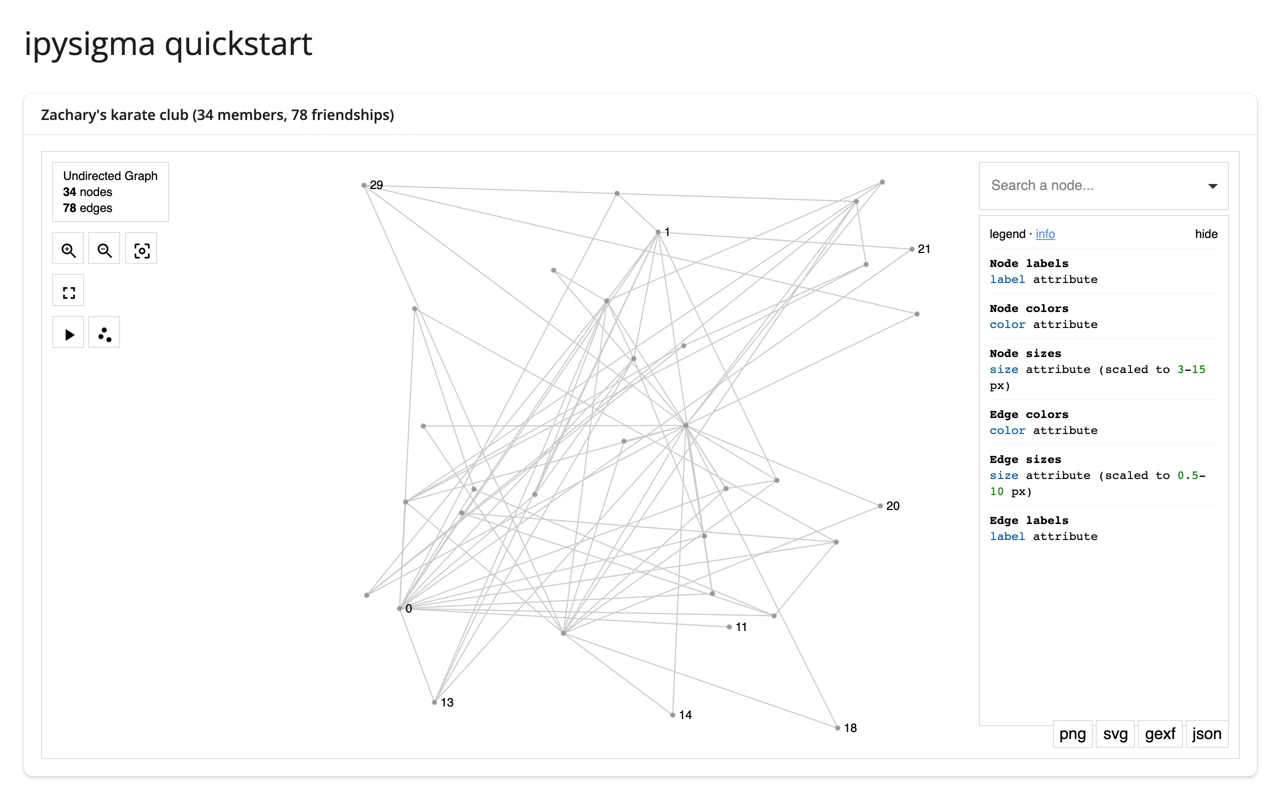
Returning a bare graph gets you search, zoom controls, a legend placeholder, and export buttons for free. For any visual encoding, construct a Sigma(...) instead, as every other example in this guide does.
What you can build
Data-driven node color and size
Node attributes become visual variables by name; a DegreeView (or any {node: value} mapping) works directly for numeric channels like size.
    @render_ipysigma
    def graph():
        # node_color/node_size read straight from node attributes (club) or a
        # DegreeView; ipysigma adds a clickable legend for the categorical color.
        return Sigma(G, node_color="club", node_size=G.degree)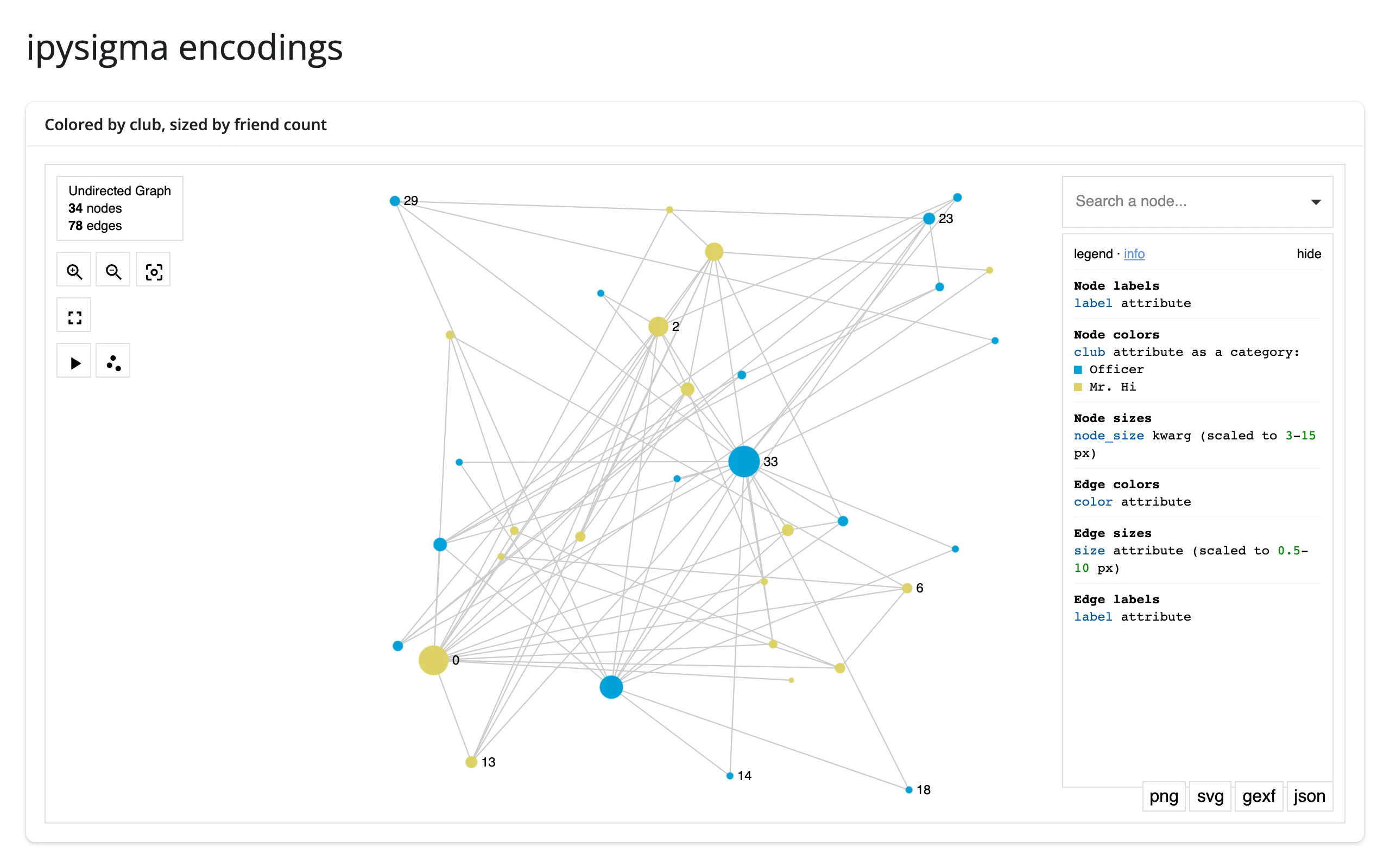
Metrics computed where they’re cheapest
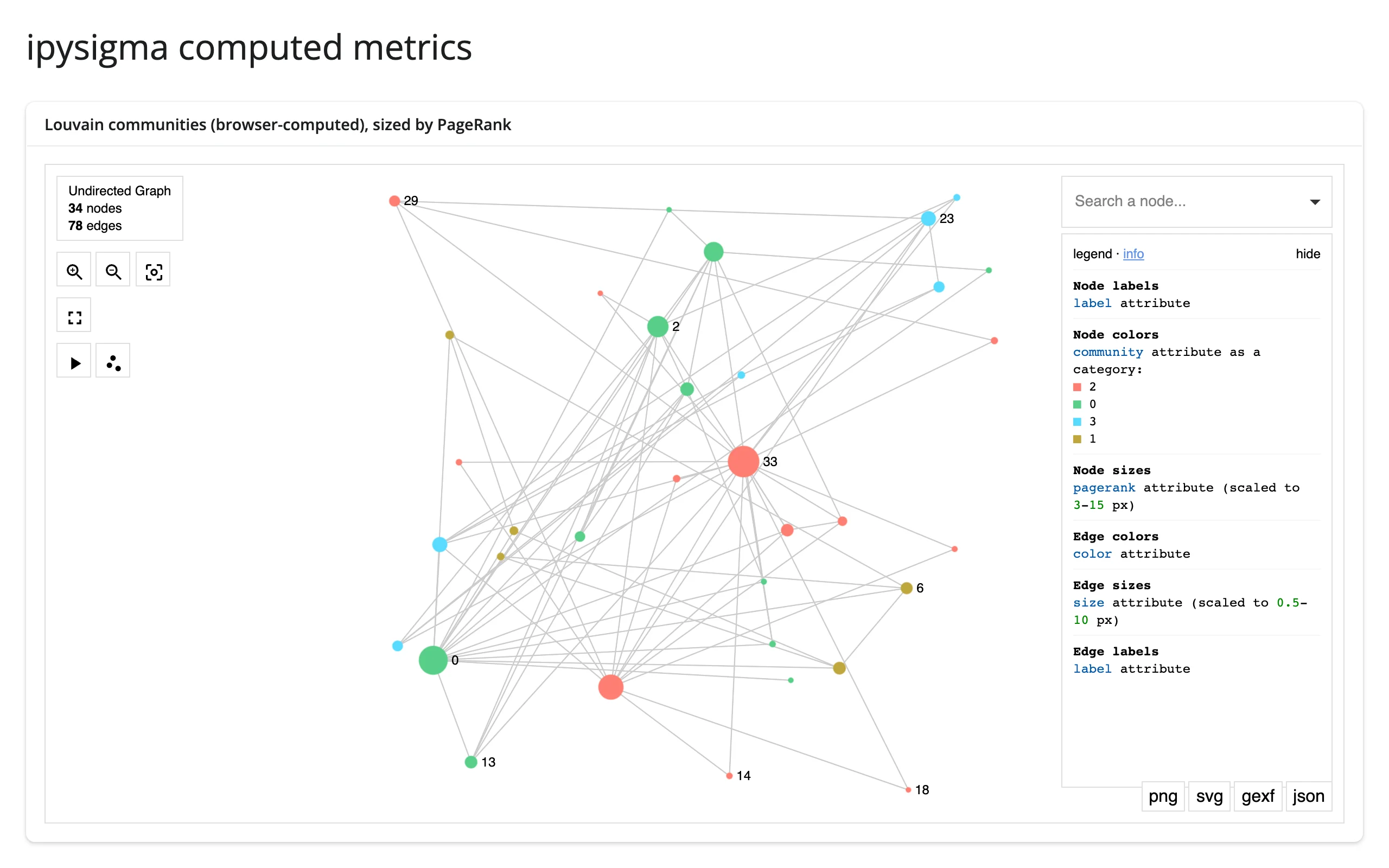
node_metrics={"community": "louvain"} runs Louvain community detection in the browser with graphology, at no Python cost. For anything else – PageRank here – compute it once in Python and set it as a node attribute.
    @render_ipysigma
    def graph():
        return Sigma(
            G,
            # Computed by graphology in the browser, not in Python
            node_metrics={"community": "louvain"},
            node_color="community",
            node_size="pagerank",
        )
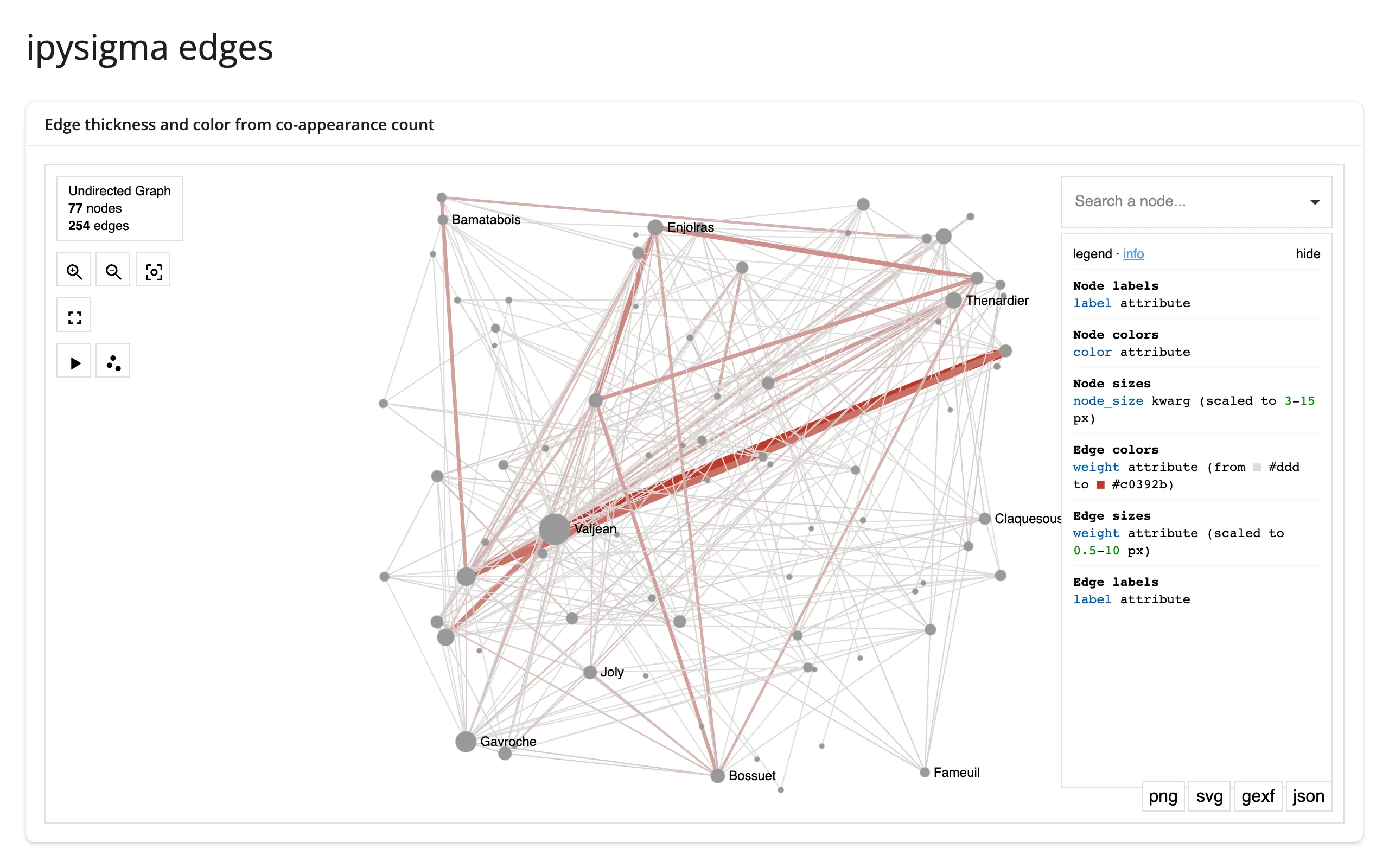
Edges carry data too
edge_color/edge_size work exactly like their node counterparts, and clickable_edges=True lets users click an edge (not just a node) to inspect it – shown in Reacting to user interaction below.
    @render_ipysigma
    def graph():
        return Sigma(
            G,
            node_size=G.degree,
            edge_size="weight",
            edge_color="weight",
            edge_color_gradient=("#ddd", "#c0392b"),
            # Lets users click an edge (not just a node) to inspect it
            clickable_edges=True,
        )
ForceAtlas2, laid out live in the browser
start_layout=<seconds> runs the ForceAtlas2 force-directed algorithm in a web worker and stops after the given time, writing the converged positions back to Python (see camera_state and layout). Prefer a number of seconds over True, which runs forever.
    @render_ipysigma
    def graph():
        # No layout= is given, so nodes start at random positions; start_layout
        # runs ForceAtlas2 in a web worker for 4 seconds, then stops and writes
        # the converged positions back to the `layout` trait.
        return Sigma(G, start_layout=4, node_size=G.degree)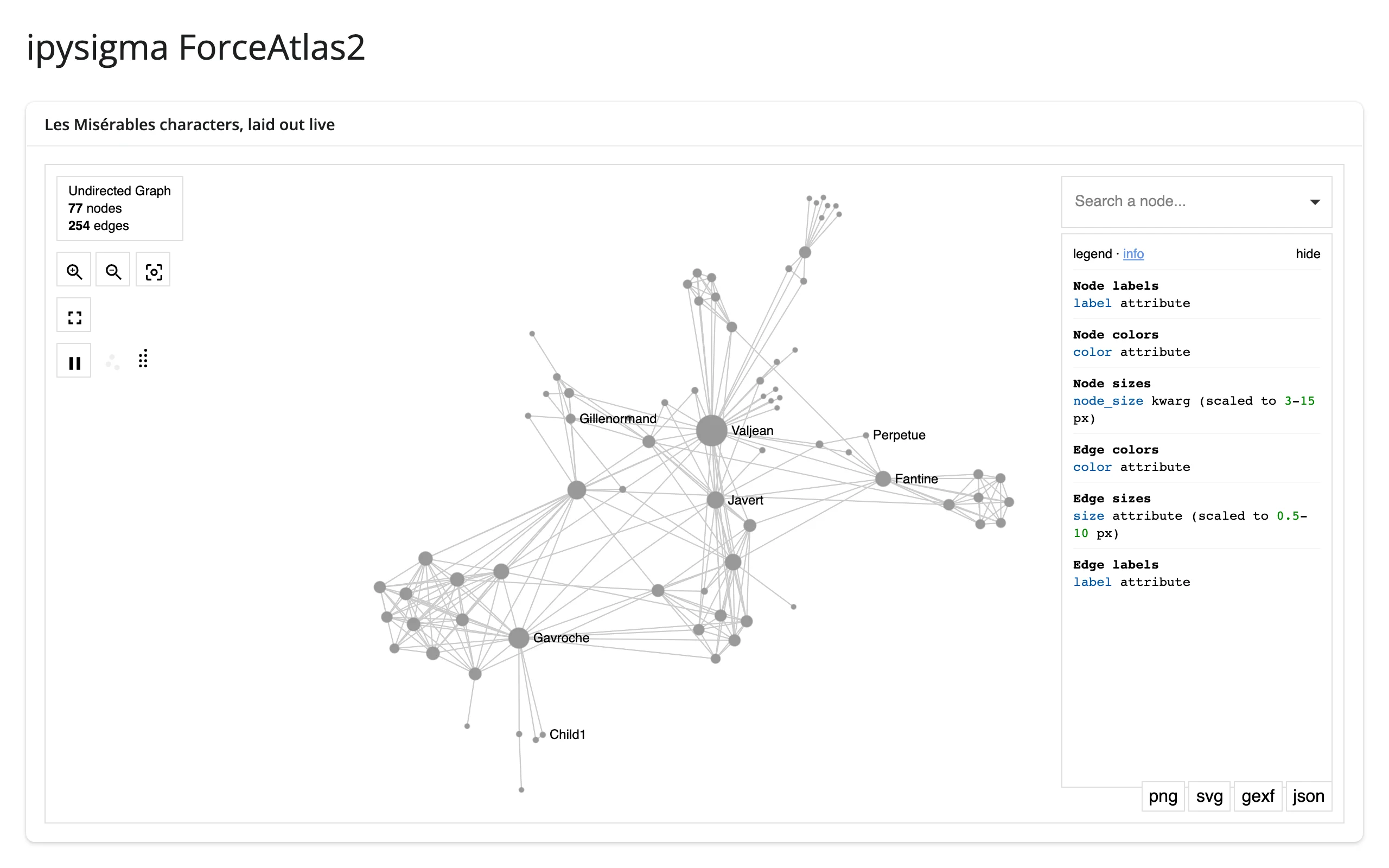
Scale: tens of thousands of nodes
sigma.js draws on the GPU, so it stays interactive well past where SVG-based graph libraries bog down. Passing precomputed layout= positions (rather than letting ipysigma lay the graph out) avoids both the random-hairball first frame and a full position write-back to Python on first render.
    @render_ipysigma
    def graph():
        return Sigma(
            G,
            layout=layout,
            node_color="cluster",
            default_node_size=2,
            hide_edges_on_move=True,  # keeps panning smooth at this size
        )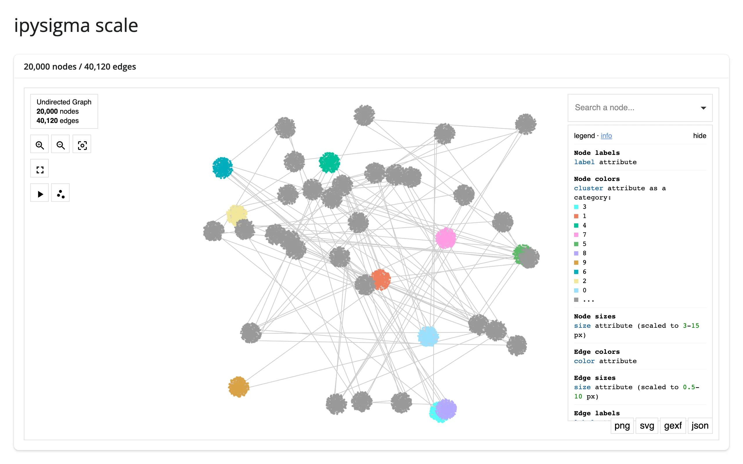
40 synthetic clusters, 20,000 nodes, ~40,000 edges, panned and zoomed smoothly in testing. The legend caps categorical colors at 10 by default (max_categorical_colors) – the other 30 clusters here render gray, which is correct behavior worth knowing about before you wonder where your colors went.
Reacting to user interaction
render_ipysigma declares no reactive accessor methods – there’s no graph.selected(). Every interaction instead goes through graph.read("<trait>"), which reads a synced ipywidgets trait of the rendered Sigma the same way reactive_read(graph.widget, "<trait>") would (see the reacting to widgets article for why .read() is the taught way to reach for that now). The traits below are the ones a real gesture actually changes; graph.widget.trait_names() lists many more (mostly write-only rendering options you pass to Sigma() at construction instead).
Traits worth reading
| trait | returns | fires when | None/[] means |
default rate policy |
|---|---|---|---|---|
selected_node |
str \| None |
clicking a node, choosing one in the search box, or in-graph search | nothing selected (also clears when an edge or stage is clicked) | not rate-limited |
selected_edge |
(str, str) \| None |
clicking an edge (requires clickable_edges=True) |
nothing selected (also clears when a node is clicked) | not rate-limited |
selected_node_category_values |
list \| None |
clicking a swatch in the legend | []/None: no filter, every category shown |
not rate-limited |
camera_state |
dict (x, y, ratio, angle) |
panning or zooming | n/a – always has a value | not rate-limited |
layout |
dict[node, {"x", "y"}] \| None |
once at mount, and again whenever ForceAtlas2 (start_layout) stops |
None until the first layout exists |
not rate-limited |
snapshot |
str (PNG data URL) \| None |
after you send {"msg": "render_snapshot"} (there’s no browser gesture for it) |
no snapshot captured yet | not rate-limited |
selected_node is always a str, even for integer node keys (int(graph.read("selected_node")) or graph.widget.get_selected_node(), which converts back to the original key type – call it only after you’ve already taken a reactive dependency via .read(), since it doesn’t take one itself).
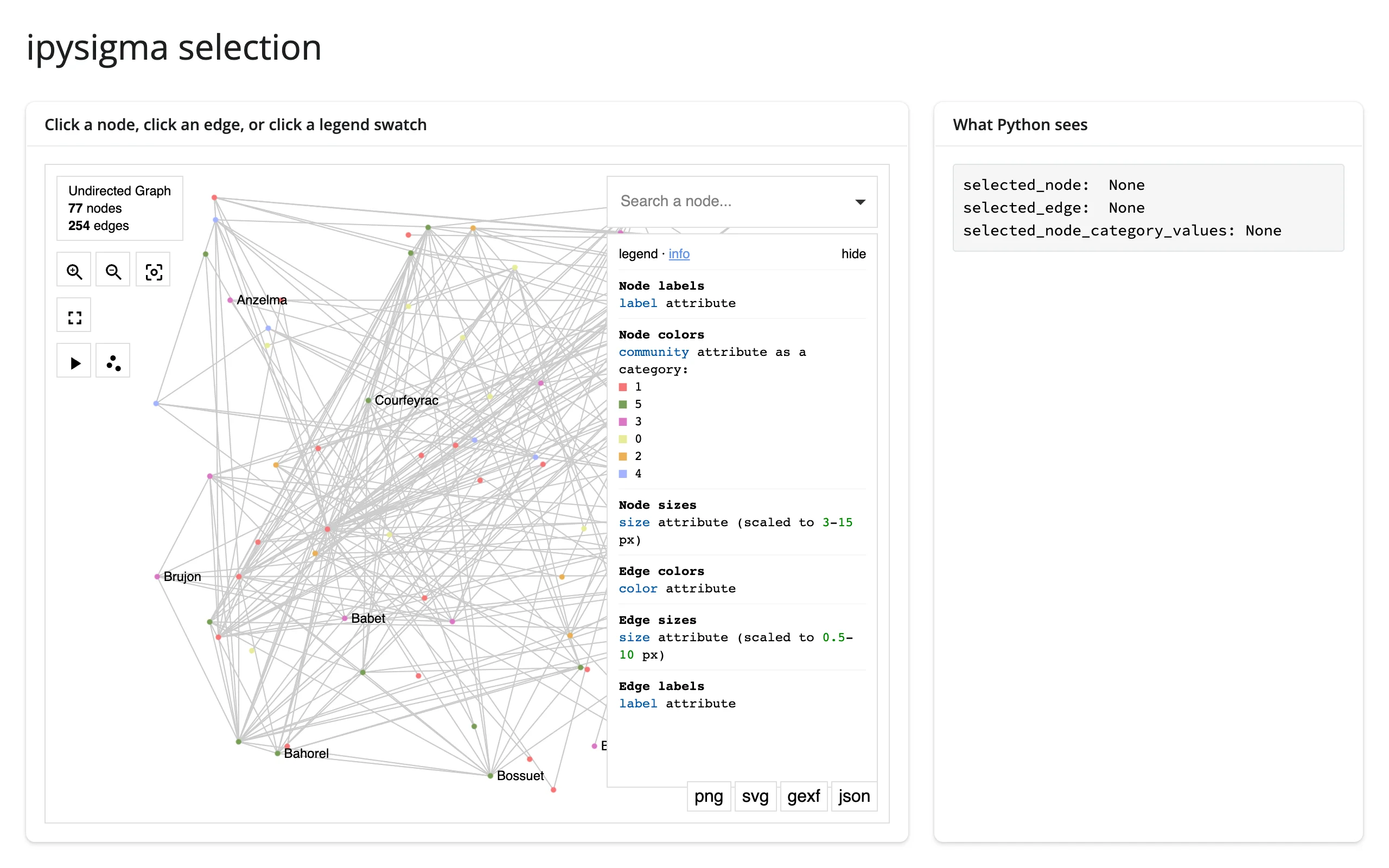
Selecting nodes, edges, and the legend
Node and edge selection are mutually exclusive (selecting one clears the other); the legend’s category filter is independent of both and persists across node/edge clicks.
        @render.code
        def state():
            node = graph.read("selected_node")
            edge = graph.read("selected_edge")
            categories = graph.read("selected_node_category_values")
            return (
                f"selected_node:  {node!r}\n"
                f"selected_edge:  {edge!r}\n"
                f"selected_node_category_values: {categories!r}"
            )
Before any interaction, and after clicking a legend swatch (filtering to one community) and then an edge (which clears the node selection but keeps the filter):
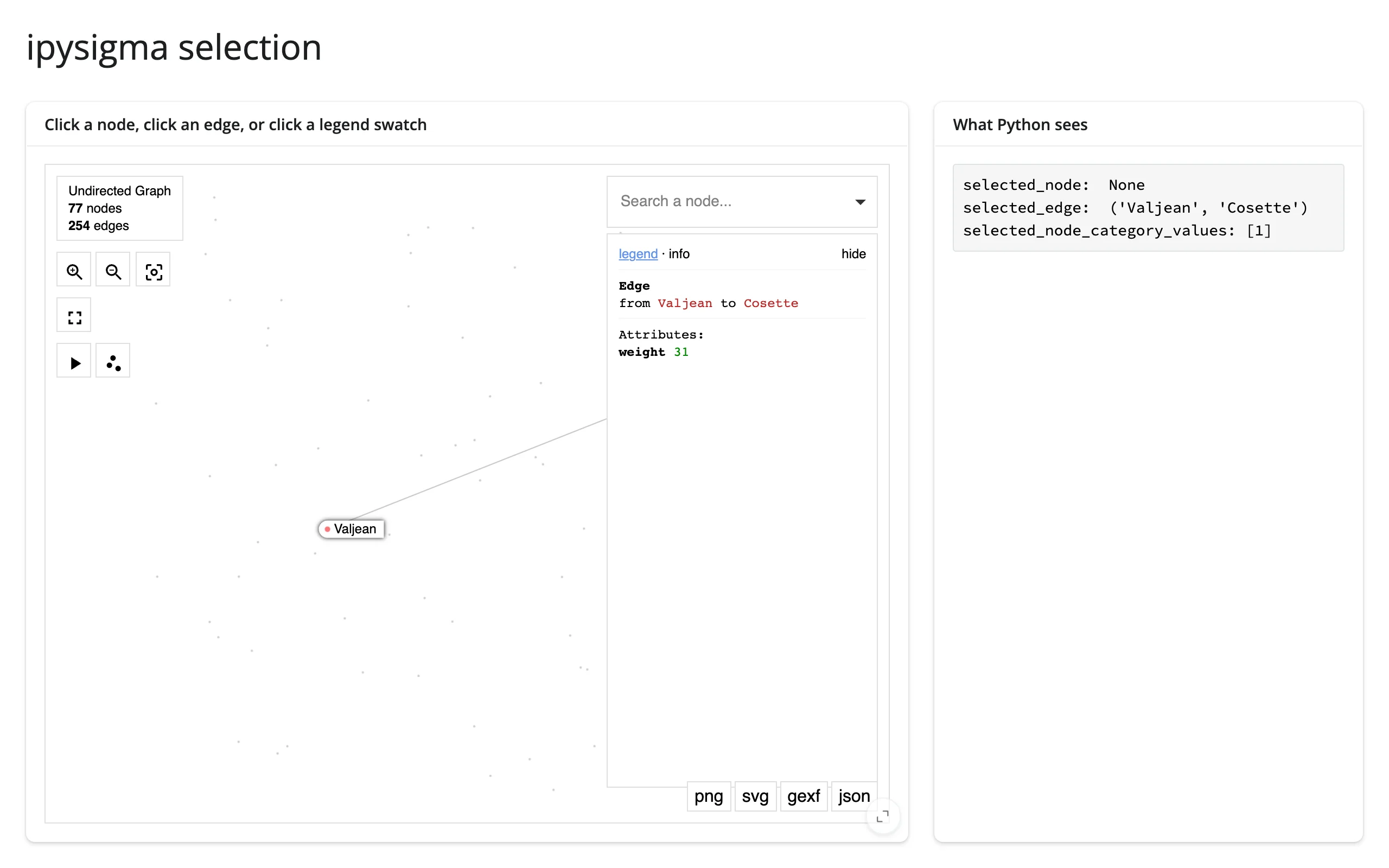
camera_state and layout
Panning, zooming, and a running start_layout all write back reactively. Positions in layout are keyed by node and already match the coordinate space you’d pass back into a new Sigma(..., layout=...).
        @render.code
        def state():
            camera = graph.read("camera_state")
            layout = graph.read("layout")
            n_positioned = 0 if layout is None else len(layout)
            camera_lines = "\n".join(f"  {k}: {v:.3g}" for k, v in camera.items())
            return f"camera_state:\n{camera_lines}\nlayout: {n_positioned} node positions"
Before any interaction, and after panning, zooming, and letting the 3-second start_layout finish:
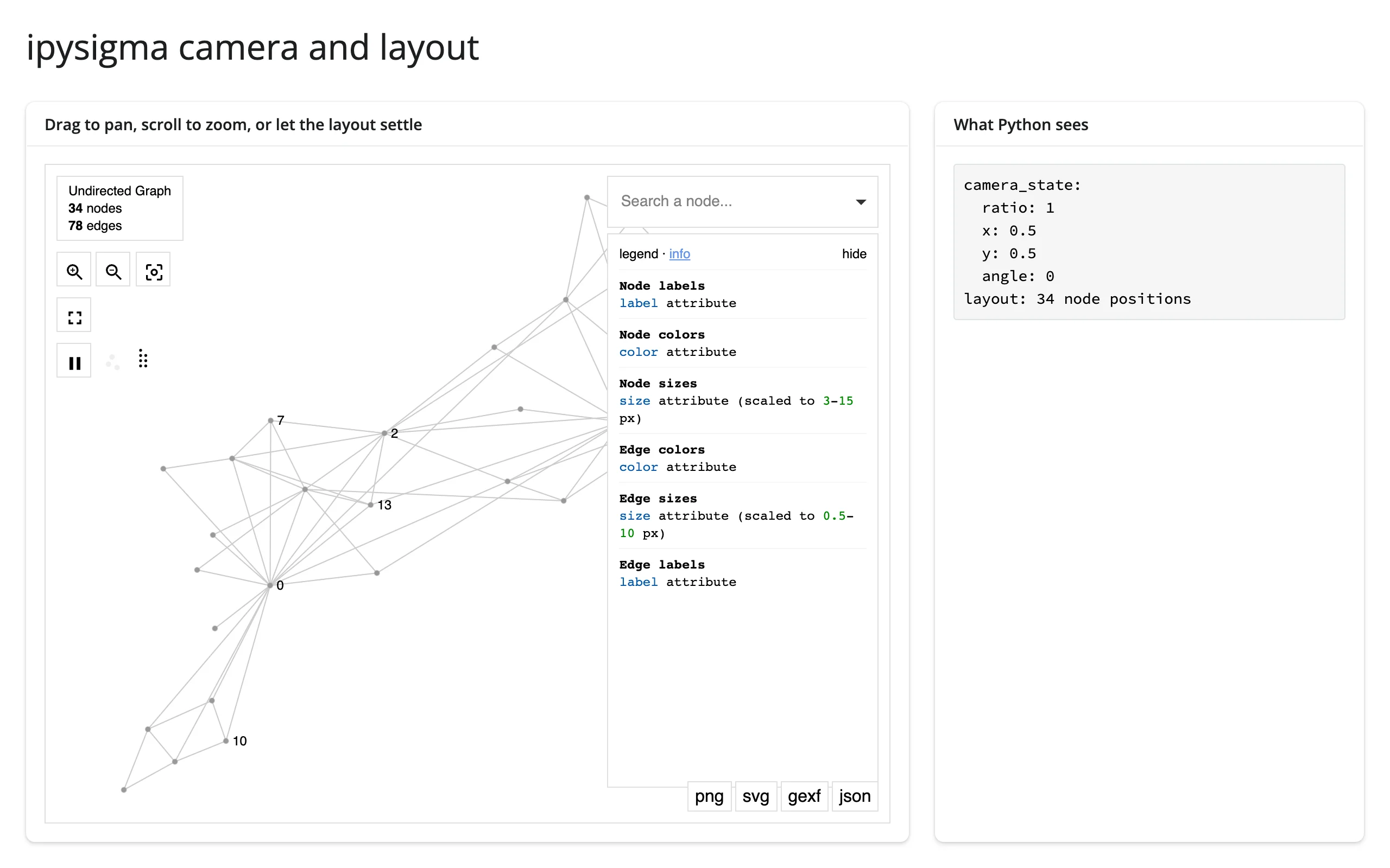
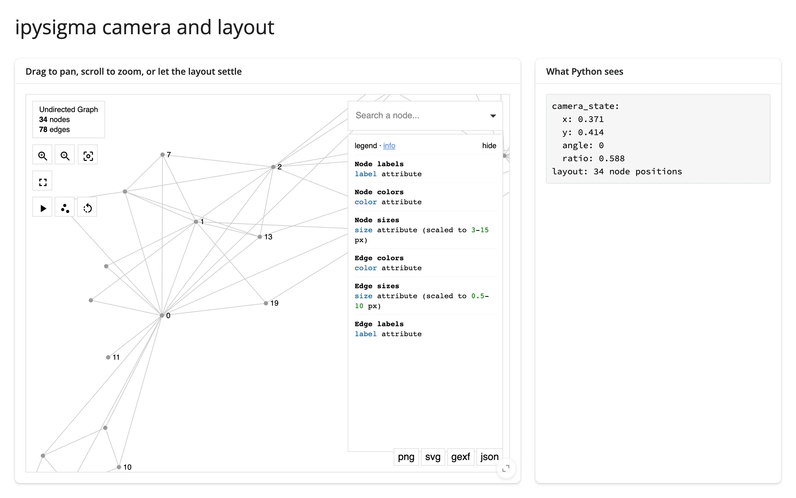
Snapshot: asking the browser for a picture
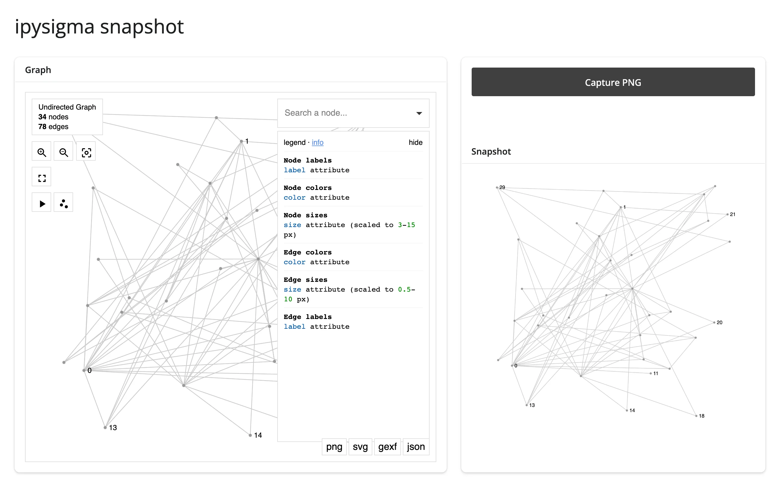
ipysigma accepts exactly one command from Python: sending {"msg": "render_snapshot"} makes the browser render a PNG and write it to the snapshot trait as a data URL, which .read("snapshot") picks up like any other trait change.
        @reactive.effect
        @reactive.event(input.snap)
        def _request_snapshot():
            # The only Python -> browser command ipysigma exposes: it answers
            # by setting the `snapshot` trait to a PNG data URL.
            graph.widget.send({"msg": "render_snapshot"})

        @render.ui
        def png():
            data_url = graph.read("snapshot")
            if data_url is None:
                return ui.p("No snapshot yet -- click the button.")
            return ui.img(src=data_url, style="max-width: 100%;")
Before capturing, and after clicking “Capture PNG”:
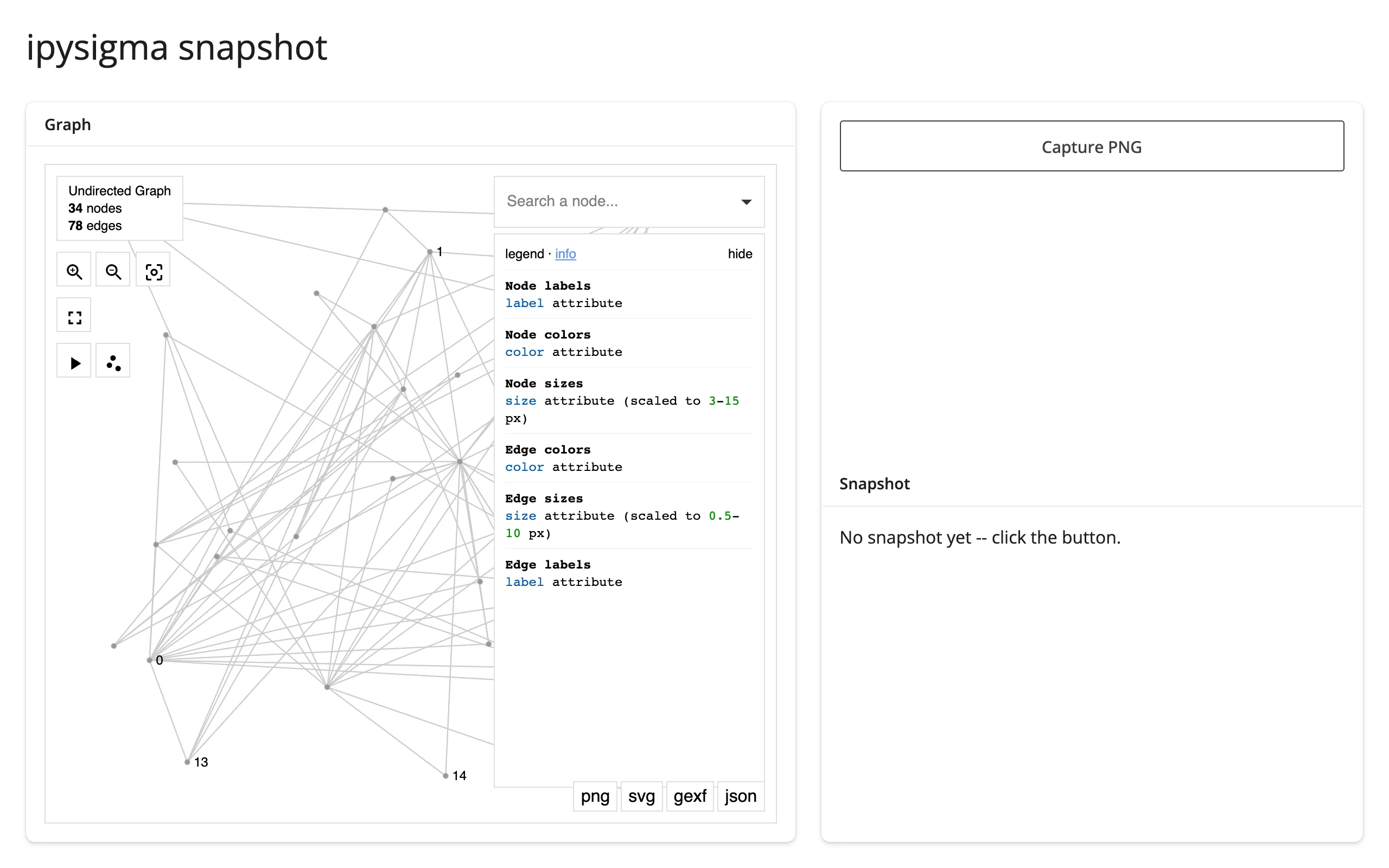
Rate limiting
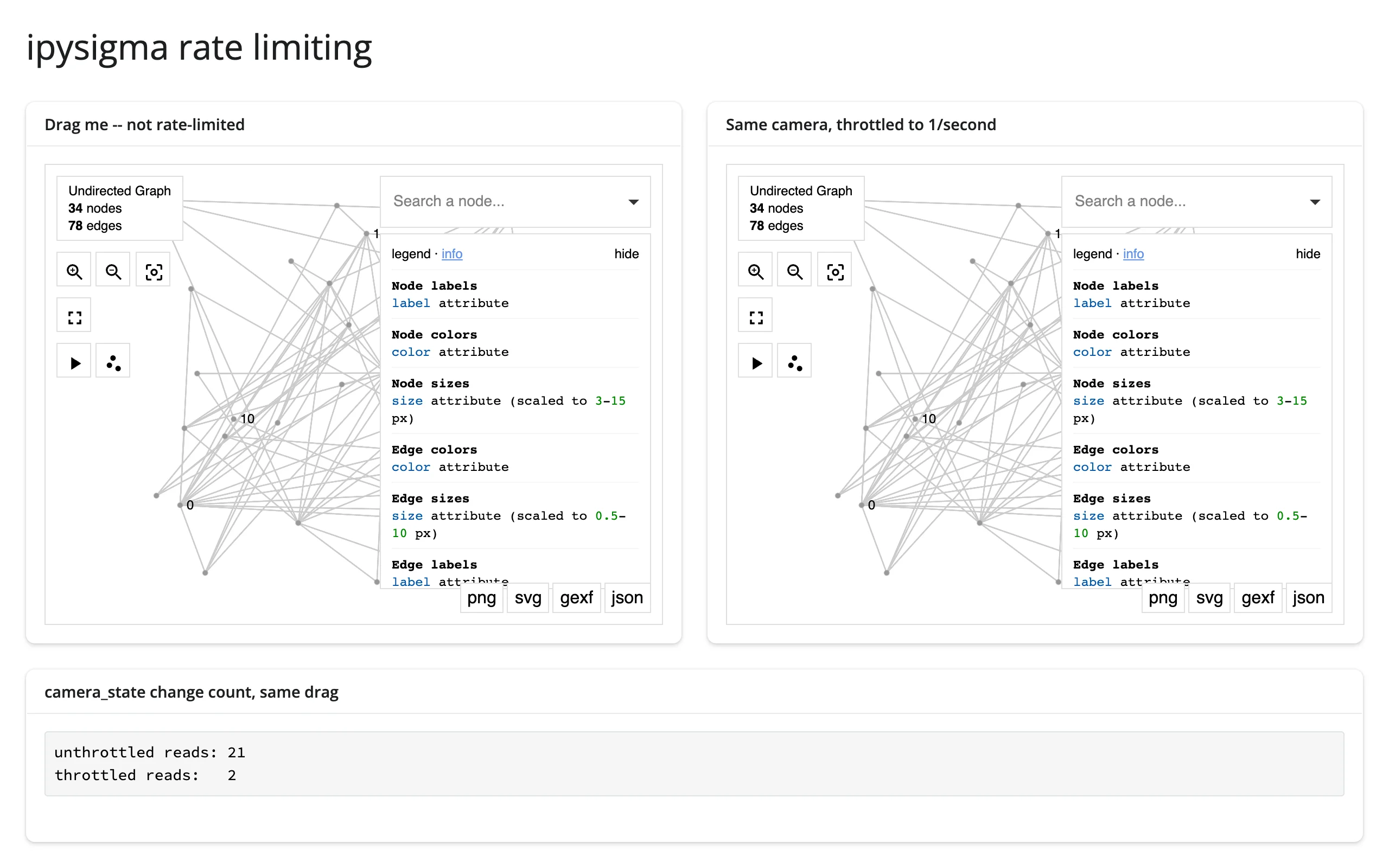
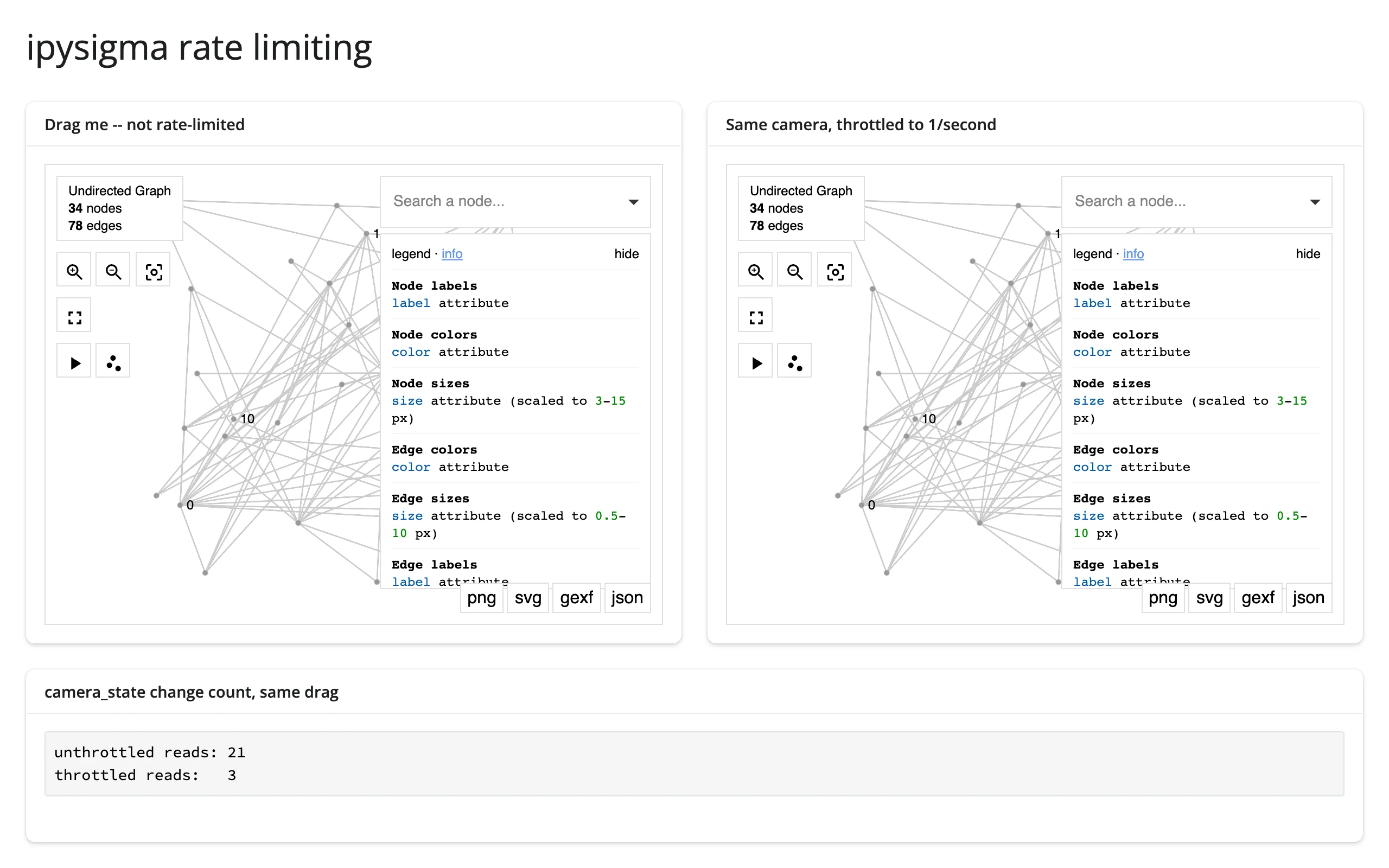
rate_policy/rate_delay on @render_ipysigma rate-limit .read()/reactive_read() for every trait on that widget (not a per-trait setting), the same as every other renderer’s .read() tier. Verified on current main: ipysigma’s own camera sync is already coarse under normal use – a continuous ~4-second drag with 60 intermediate mouse positions produced only 1-2 raw camera_state changes on the model, so a real pan/zoom rarely gives rate_policy much to smooth. It matters when something else produces a genuine burst of changes close together (the example below simulates one directly on the model to demonstrate it) or when the downstream computation a read triggers is expensive enough that even ipysigma’s own cadence is too frequent.
with ui.layout_columns(col_widths=[6, 6]):
    with ui.card(full_screen=True):
        ui.card_header("Drag me -- not rate-limited")

        @render_ipysigma
        def unthrottled():
            return Sigma(G, sync_key="cam")

    with ui.card(full_screen=True):
        ui.card_header("Same camera, throttled to 1 read per 2 seconds")

        @render_ipysigma(rate_policy="throttle", rate_delay=2)
        def throttled():
            return Sigma(G, sync_key="cam")
20 rapid, distinct camera_state changes mirrored to both widgets (sync_key keeps their cameras identical): the unthrottled counter keeps pace; the throttled one, capped to one read per 2 seconds, falls behind during the burst and catches up once it settles:
Updating the widget from Python
ipysigma reads its constructor options once, when the graph is first drawn, and registers no listeners for later trait changes – verified on current main: setting graph.widget.selected_node = "5" from an effect does reach the browser’s copy of the model (graph.read("selected_node") sees the new value), but nothing changes on screen, the same as the class docstring says. There’s no in-place update path here, unlike widgets that mirror trait changes into their view (plotly, itables’ .update()).
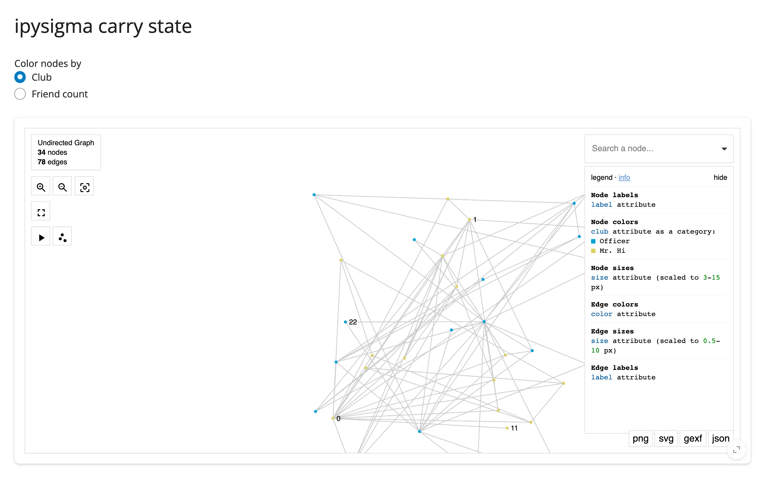
The practical pattern is to re-render, carrying forward whatever state you don’t want to lose – typically camera_state (and layout, if a layout has already converged) – by mirroring it into a reactive.value with an effect, then feeding it back into the next Sigma(...):
    camera = reactive.value({"x": 0.5, "y": 0.5, "ratio": 1, "angle": 0})

    @reactive.effect
    def _track_camera():
        req(graph.widget)
        camera.set(graph.read("camera_state"))

    @render_ipysigma
    def graph():
        color_by = input.color_by()
        with reactive.isolate():
            # isolate(): reading .widget here (not just camera) would create a
            # circular dependency on this render's own previous output
            cam = camera.get()
        if color_by == "club":
            return Sigma(G, node_color="club", camera_state=cam)
        return Sigma(
            G,
            node_color=dict(G.degree()),
            node_color_gradient=("#dbe9f6", "#08306b"),
            camera_state=cam,
        )
Switching color schemes rebuilds the graph entirely, but the zoomed-in view from before the switch is preserved exactly:
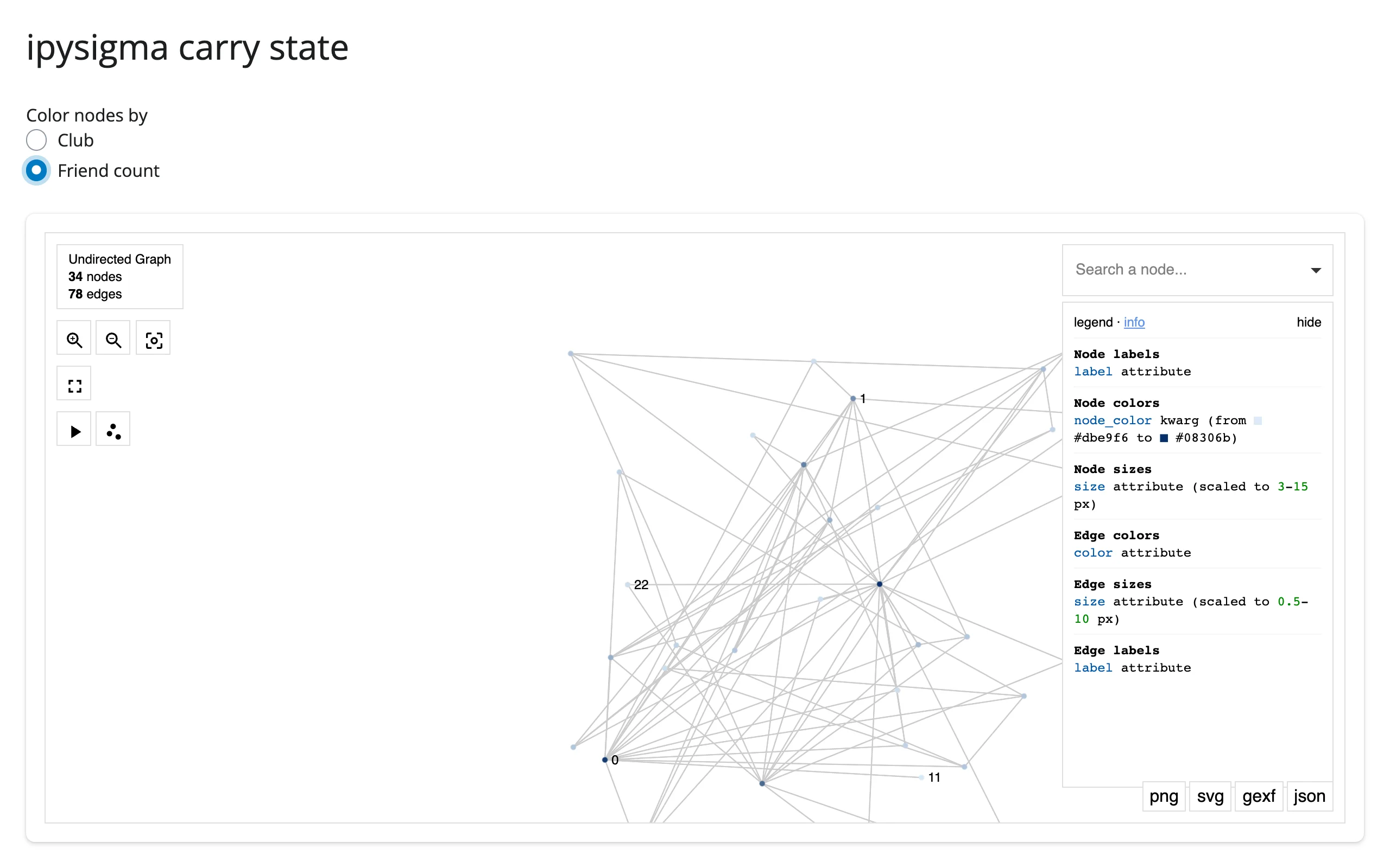
Don’t read graph.widget inside graph() itself without reactive.isolate() – before the first render, that raises req(False) and cancels the output silently. Mirroring into a reactive.value via a separate effect (as above) sidesteps this.
Coordinating multiple views
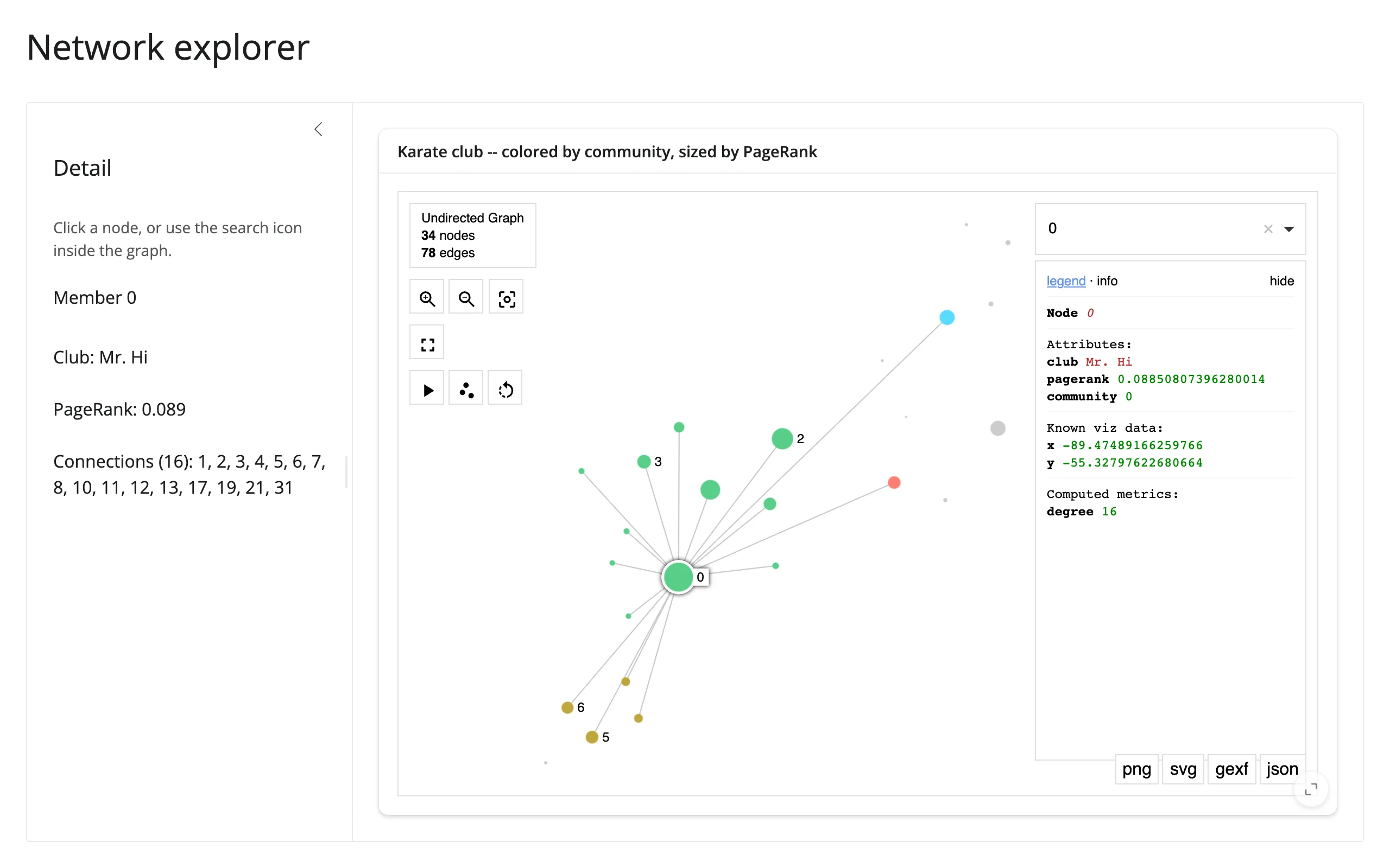
Click a node for a detail card
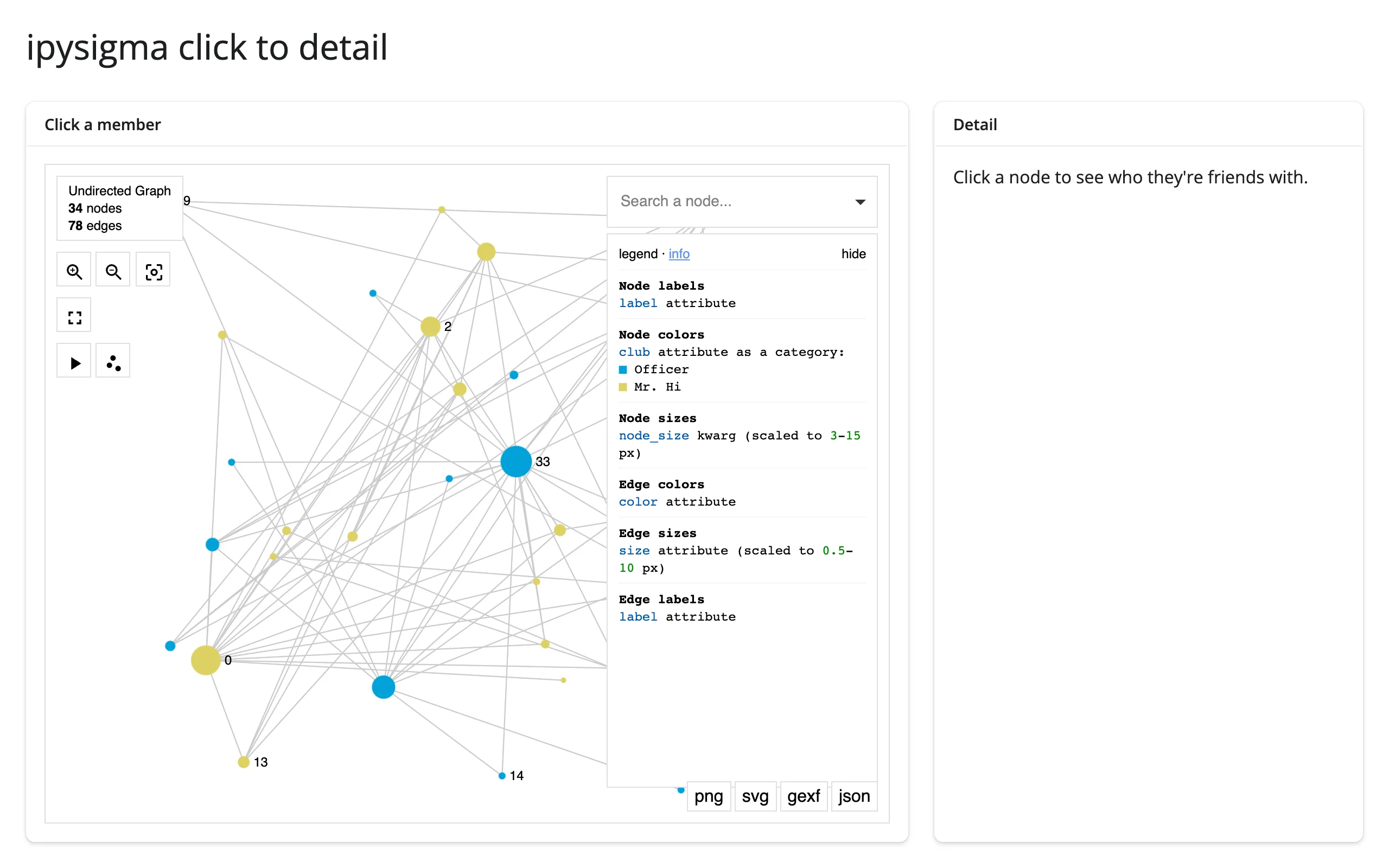
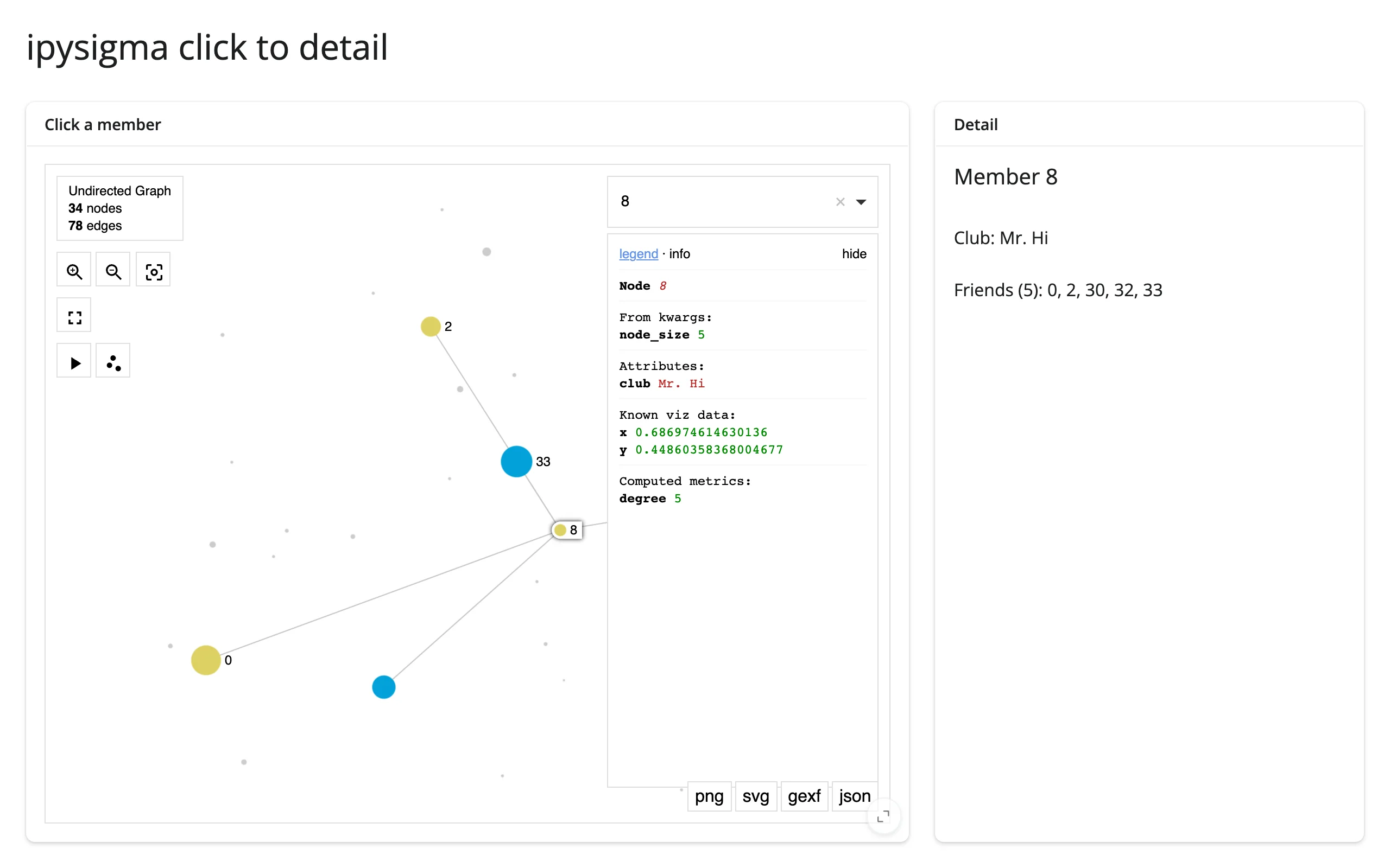
The most common pattern: read selected_node in a @render.ui and handle the “nothing selected” case for first load.
        @render.ui
        def detail():
            raw = graph.read("selected_node")
            if raw is None:
                return ui.p("Click a node to see who they're friends with.")
            node = int(raw)  # selected_node is always a string
            friends = sorted(G.neighbors(node))
            return ui.TagList(
                ui.h5(f"Member {node}"),
                ui.p(f"Club: {G.nodes[node]['club']}"),
                ui.p(f"Friends ({len(friends)}): {', '.join(map(str, friends))}"),
            )
Click a node to filter a table
Same read, different downstream view – a selected node’s neighbors as a data frame instead of prose.
        @render.data_frame
        def neighbor_table():
            raw = graph.read("selected_node")
            req(raw)
            neighbors = sorted(G.neighbors(int(raw)))
            return members[members["member"].isin(neighbors)].reset_index(drop=True)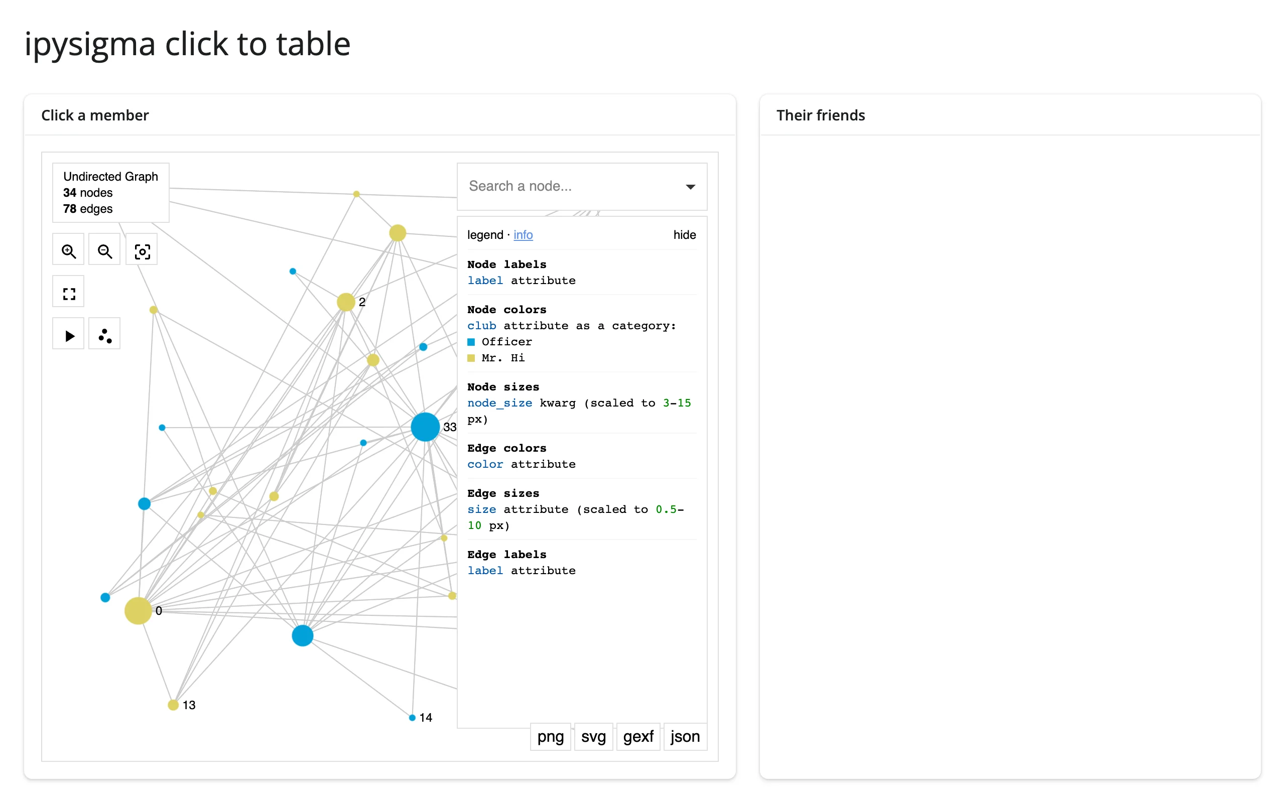
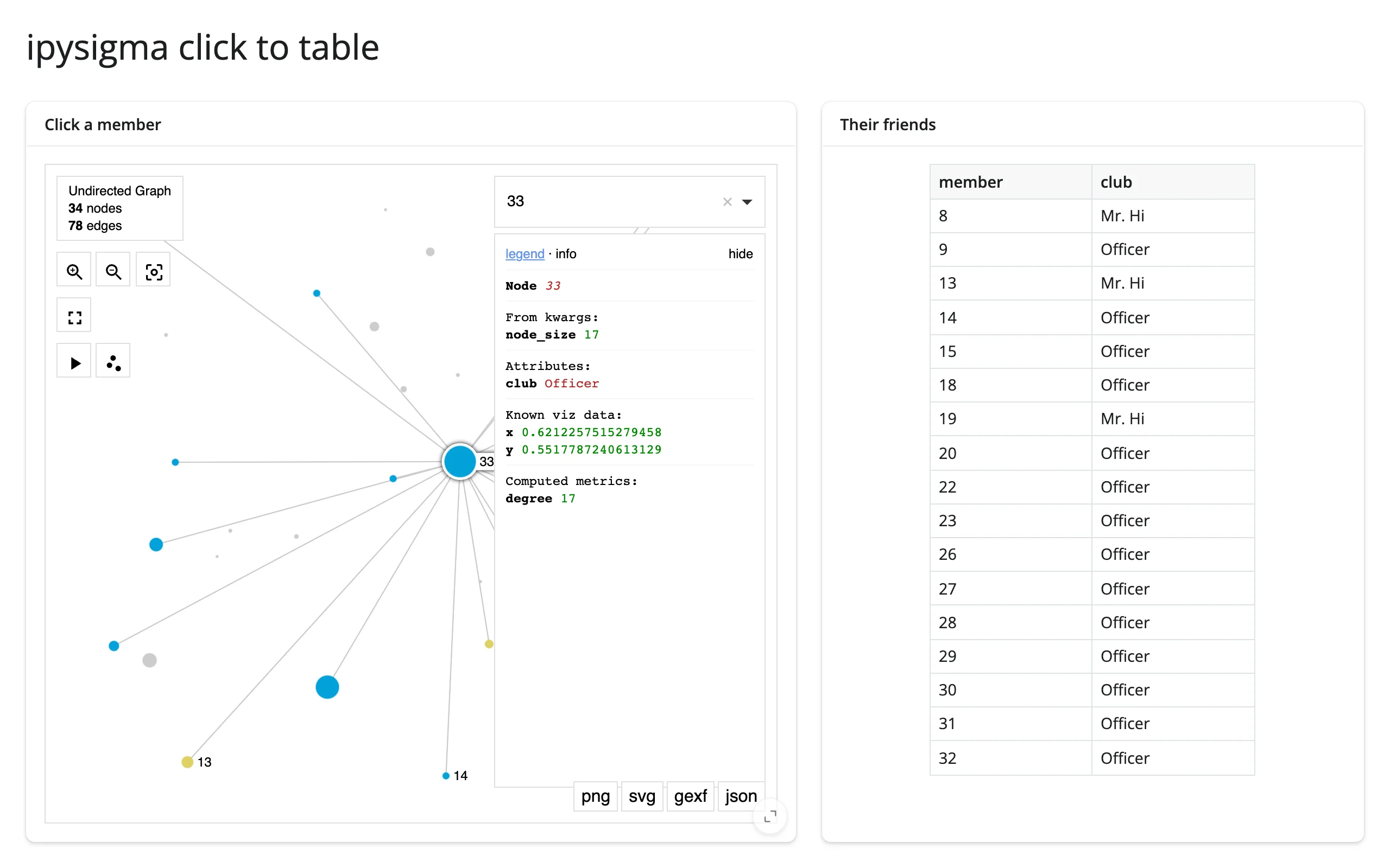
(Pairs well with itables or reactable for a richer table than render.data_frame.)
Two linked views, no Python in the loop
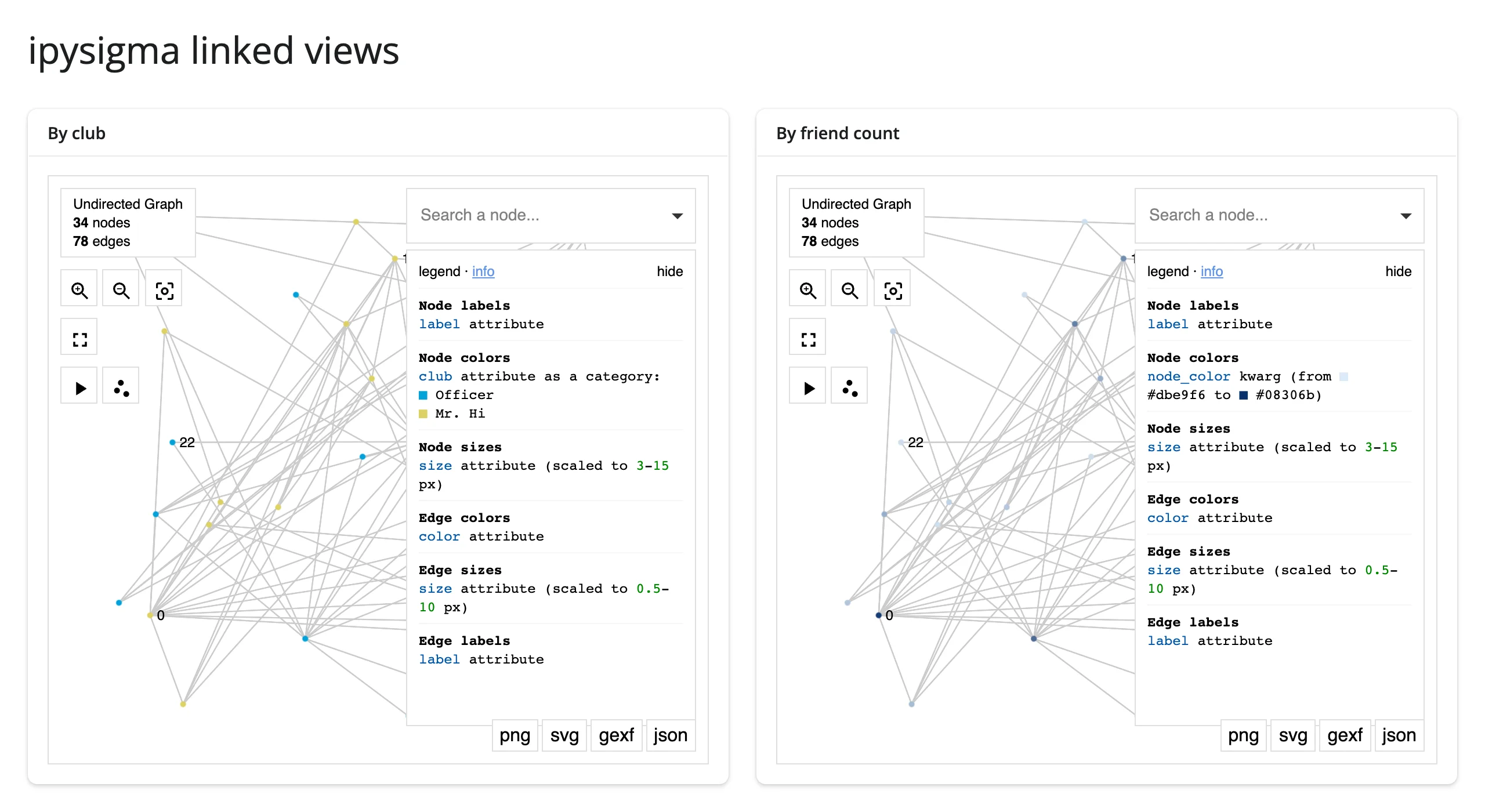
Give two Sigmas the same sync_key and the browser keeps their camera, selection, and hover in sync directly – each still reports its own selected_node to Python, so both update together with no effect wiring at all. This is the Shiny replacement for ipysigma’s SigmaGrid (a Jupyter-only small-multiples helper that isn’t a widget and can’t be returned from a render function).
with ui.layout_columns(col_widths=[6, 6]):
    with ui.card(full_screen=True):
        ui.card_header("By club")

        @render_ipysigma
        def by_club():
            # sync_key links pan/zoom/selection/hover between every Sigma that
            # shares it, even across separate outputs
            return Sigma(G, node_color="club", sync_key="karate")

    with ui.card(full_screen=True):
        ui.card_header("By friend count")

        @render_ipysigma
        def by_degree():
            return Sigma(
                G,
                node_color=dict(G.degree()),
                node_color_gradient=("#dbe9f6", "#08306b"),
                sync_key="karate",
            )
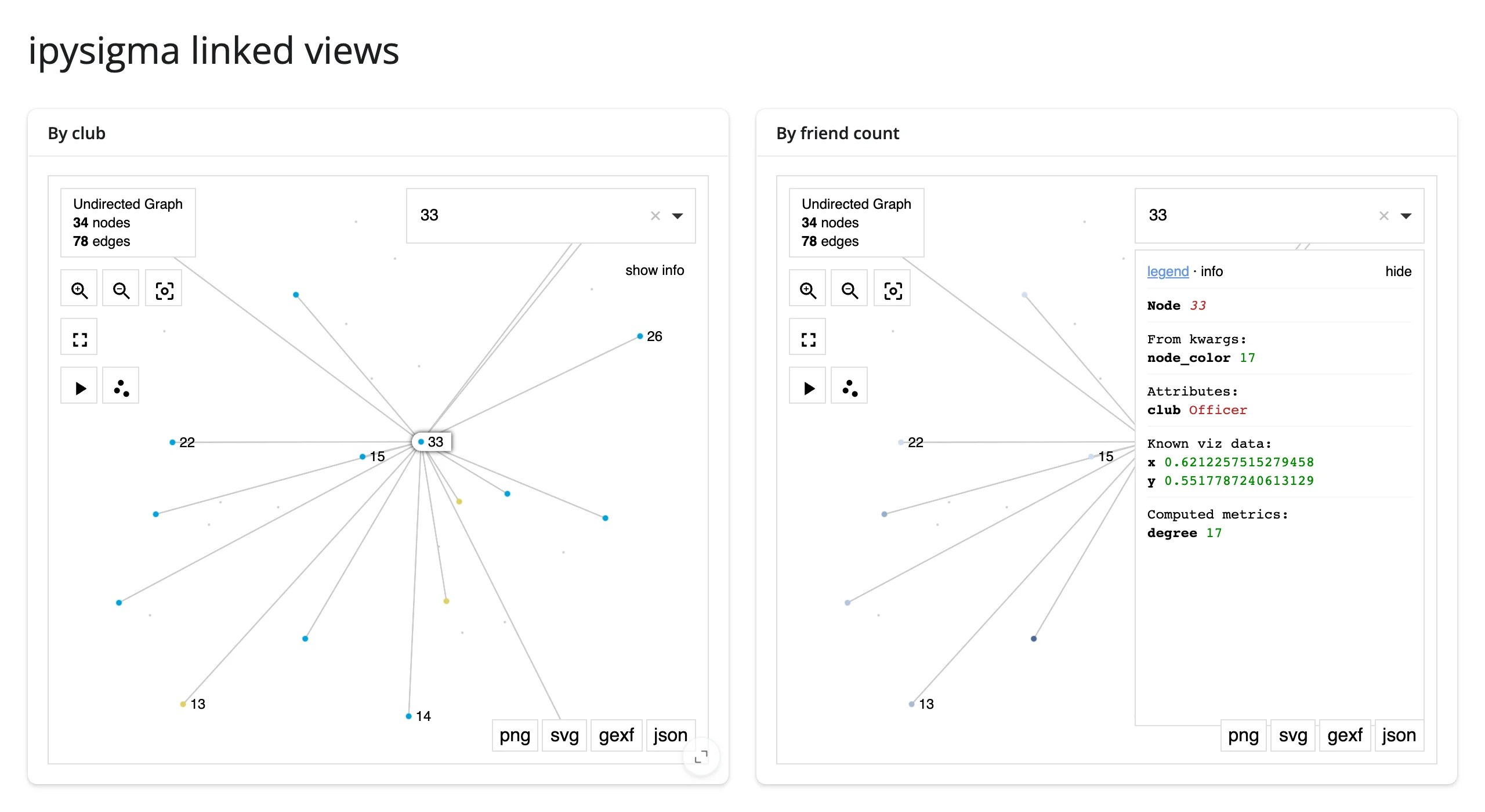
Clicking node 33 in the left graph selects it in both, including the right graph’s detail panel:
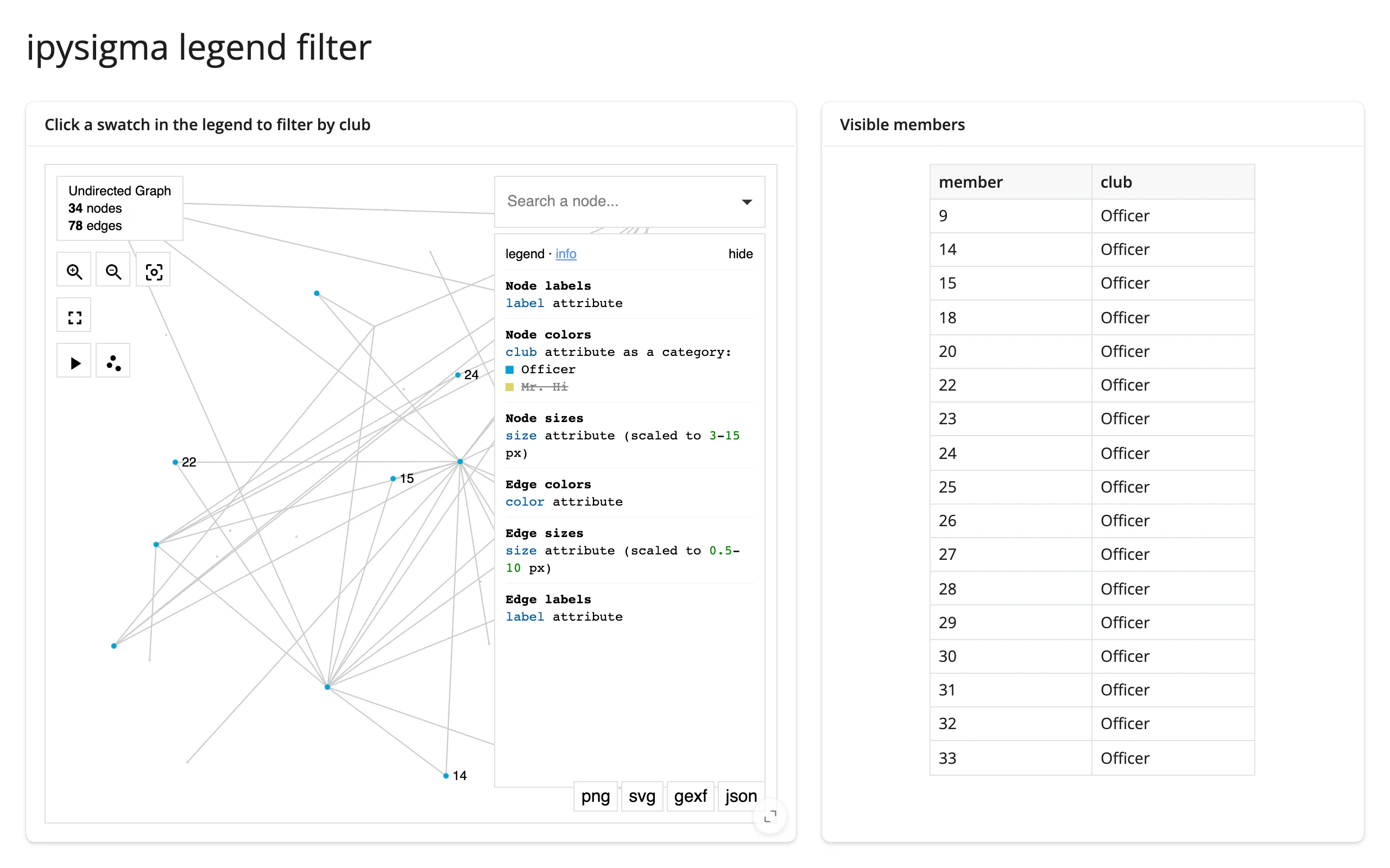
Legend click filters a table
selected_node_category_values isn’t just for dimming the graph – read it anywhere a category filter is useful.
        @render.data_frame
        def visible():
            # [] (nothing filtered) means "show everything", not "show nothing"
            categories = graph.read("selected_node_category_values")
            shown = members if not categories else members[members["club"].isin(categories)]
            return shown.reset_index(drop=True)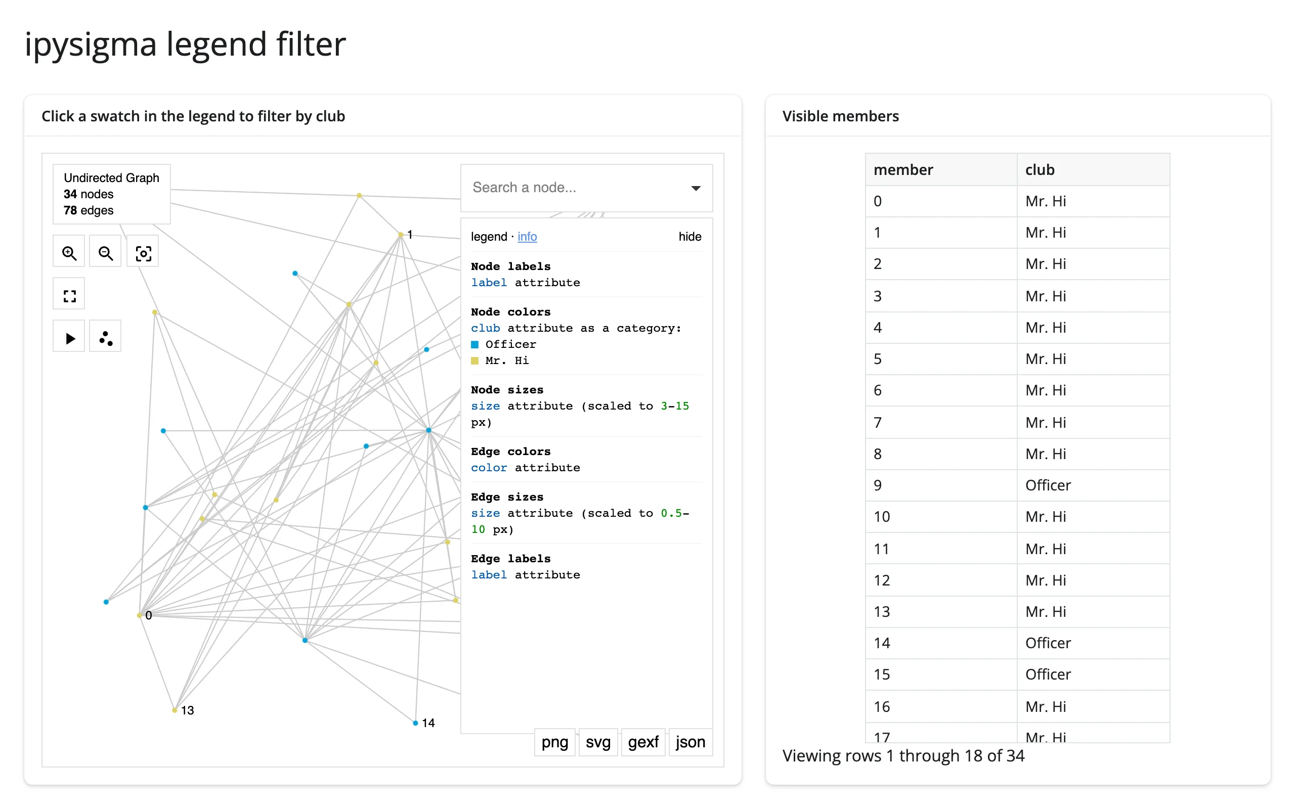
Large data
ipysigma draws with the GPU (sigma.js/WebGL), the “draw it with the GPU in the browser” approach – see Large data & performance’s three approaches. See “Scale: tens of thousands of nodes” above, under “What you can build”: 40 synthetic clusters, 20,000 nodes and ~40,000 edges panned and zoomed smoothly in testing, with precomputed layout= positions (skipping both the random-hairball first frame and a full position write-back to Python on first render). Past that scale, ipycytoscape – the sibling that renders one ipywidget per element – is the one that falls over first, not this renderer.
Layout and sizing
In a filling layout, the graph fills its container – unless the widget has an explicit height/raw_height (a height of 500px, sigma’s default, or one set globally with Sigma.set_defaults(height=...), still counts as “unset” and fills). output_widget(..., fillable=False) – a container with no definite height – falls back to sigma’s 500px default rather than collapsing to 0, fixed since the earlier PR-era evaluation (docs/widget-reports/ipysigma/) and reverified here (make test-playwright ×7, current main).
full_screen=True cards and ipysigma’s own fullscreen button both work and restore the prior size on exit. The 250px info/legend panel eats into a narrow card’s width – pass hide_info_panel=True if you’re embedding a small graph. The info panel can also visually overlap the canvas in a narrow container (it’s absolutely positioned on top), which only matters if you’re scripting clicks against it, not for normal use.
Gotchas and limitations
Verified on current main (shinywidgets, ipysigma 0.24.6, networkx 3.7):
- Keep to about 5 ipysigma graphs on one page. Each
Sigmaview uses 3 WebGL contexts (confirmed: 2 views measured 6 WebGL + 8 2D canvases total), and browsers cap live contexts at roughly 16 per page. Past that, the browser evicts the oldest contexts, blanking whichever graphs were already on the page – a sigma.js/ browser limit, not specific to Shiny’s re-rendering. Re-rendering one graph no longer leaks its old context (confirmed: the fullrender_ipysigmaPlaywright suite, including the dedicated re-render/context-release tests, passes on current main), so the remaining constraint is the simultaneous-graphs-per-page ceiling itself. - No Python -> browser trait sync. Setting
graph.widget.selected_node,.camera_state, or any other trait from Python updates the ipywidgets model (sograph.read()sees the new value) but changes nothing on screen – ipysigma reads its options once, at first draw. Re-render instead (see Updating the widget from Python). - igraph works, undocumented.
networkx_to_sigma()(the coercion behind returning a bare graph) just callsSigma(x), which accepts anigraph.Graphdirectly (ig.Graph.Famous("Zachary")renders fine) even though neither ipysigma’s nor shinywidgets’ docs mention it for this path. node_metricsonly supports"louvain". It’s not a general metrics engine – PageRank, betweenness, and everything else still need computing in Python and attaching as a node attribute first (03_computed_metrics.pydoes both side by side).- A numeric mapping for
node_coloris categorical unless you add a gradient or scale.node_color=degree_dictalone buckets values into (at most 10, by default) discrete colors; passnode_color_gradient=(...)for a continuous scale (used in11_carry_state_rerender.pyand14_linked_views_sync_key.py). Literal CSS colors (e.g., a precomputed{node: "#e41a1c"}map) belong inraw_node_color, notnode_color, which otherwise treats them as category labels needing a palette (used ingallery/showcase_stdlib_imports.py). - Node keys must be
int,str, orfloat, and not mixed.selected_nodealways comes back as astrregardless of the original key type; convert withint(...)orgraph.widget.get_selected_node()(call the latter only after a.read()on the same widget has already established the reactive dependency, sinceget_selected_node()itself doesn’t take one). SigmaGridisn’t supported. It’s a Jupyter-only display helper, not a widget, so it can’t be returned from@render_ipysigma. Use two outputs sharing async_keyinstead (see Coordinating multiple views).
Gallery candidates
gallery/template_network_explorer.py– template. Any networkx graph, Louvain-colored and PageRank-sized with zero Python graph algorithms beyond onenx.pagerank()call, plus a sidebar detail card. Swap in your own graph and detail fields.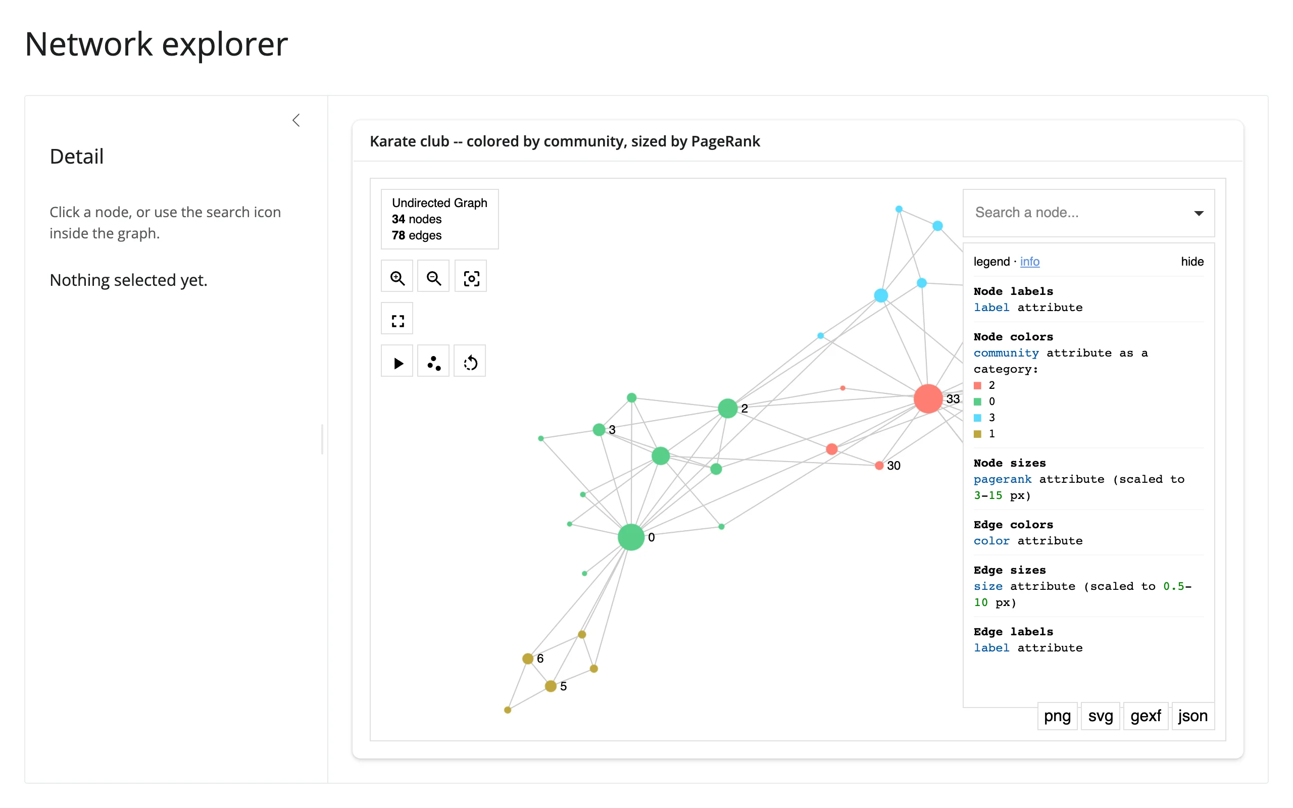
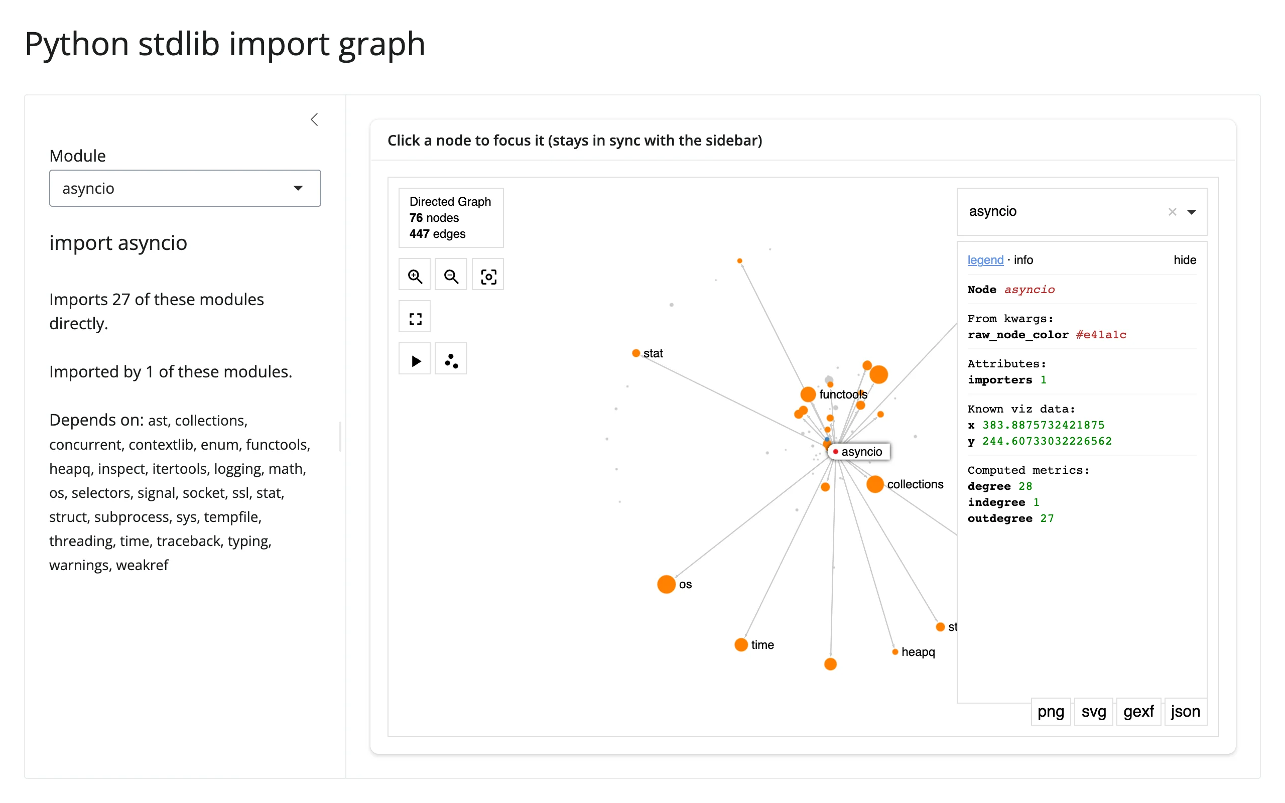
gallery/showcase_stdlib_imports.py– showcase. Python’s own standard library as an import graph (built byast-parsing ~80 modules’ source – no downloads, no network). Click a module (or pick one from the sidebar, kept in sync both ways) and the graph recolors around it: red for the focus, orange for what it imports, blue for what imports it. Demonstrates the full carry-state-across-re-render pattern – the camera doesn’t move when you click around. 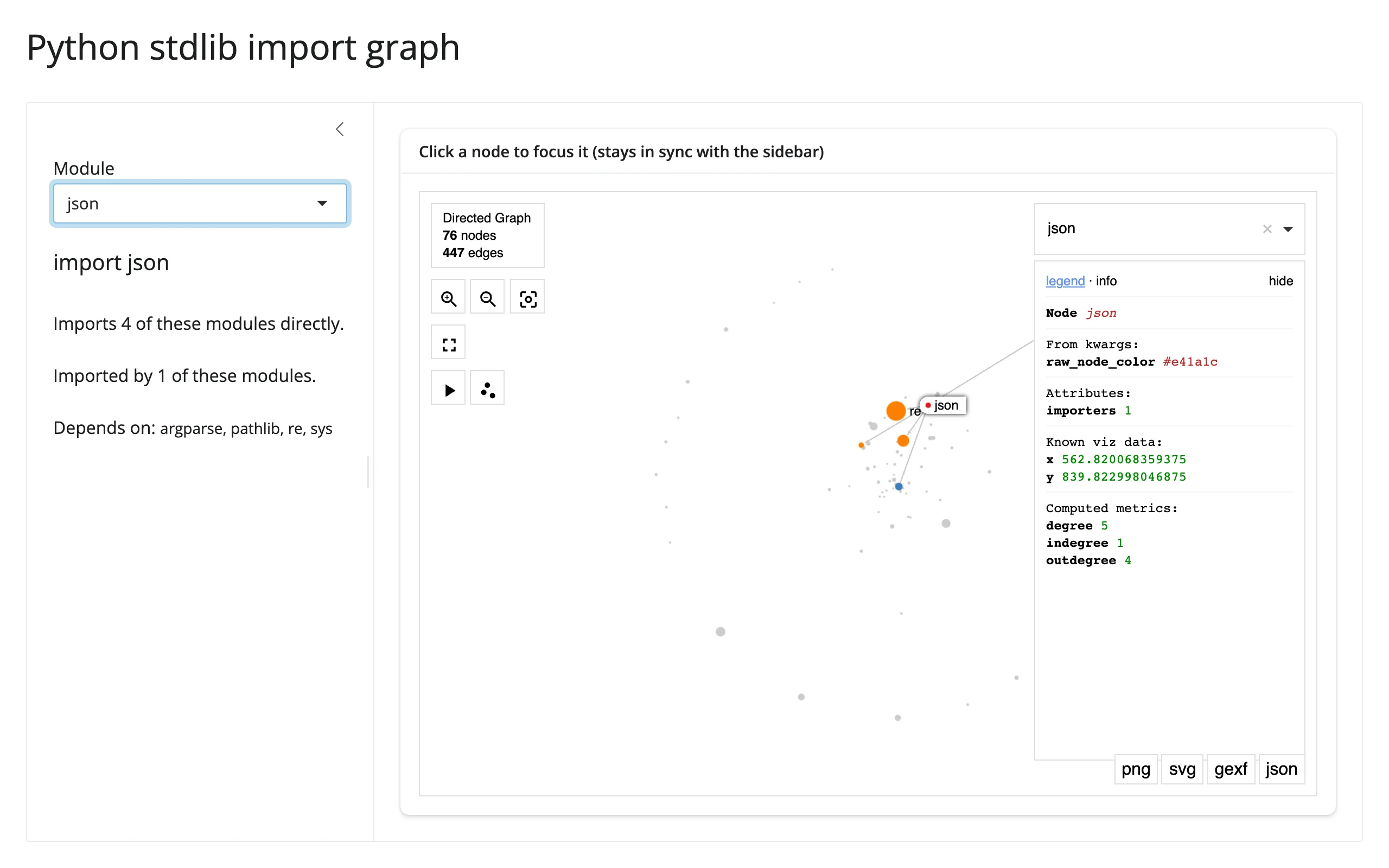
Learn more
- ipysigma on GitHub – the full
Sigma()option reference (far more than this guide covers: pictograms, halos, borders, z-index, per-edge curveness and type, and more). - sigma.js and graphology – the underlying rendering and graph-data libraries, for anyone customizing further.
- Related guides in this roster: ipycytoscape (smaller graphs, richer styling), itables and reactable (good table partners for the linked-view patterns above).