jupyter-scatter
jupyter-scatter (the jscatter package) is a WebGL scatter plot built by Fritz Lekschas on top of regl-scatterplot. Its whole reason to exist is scale: where most Python plotting libraries start to struggle in the tens or hundreds of thousands of points, jupyter-scatter stays interactive into the millions, because every point is drawn by the GPU instead of the DOM or an SVG. It also ships a real interaction model out of the box – lasso selection with modifier keys, hover tooltips with histograms, animated transitions between coordinate sets – rather than leaving you to build those on top of a bare canvas.
@render_jscatter takes a jscatter.Scatter (jupyter-scatter’s builder object) or its underlying JupyterScatter widget, and does the usual shinywidgets layout work: the plot resizes to fill its card or output, unless it has a height of its own. The renderer’s accessors turn the plot’s lasso/click selection into reactive values: .selected() is the selection as row positions, and .selected_rows() the selected rows of the plot’s data frame – so “what did the user select” reads like input.my_slider() instead of a widget trait you have to wire up by hand.
Reach for jupyter-scatter when the point count is the thing standing between you and plotly or altair – a few hundred thousand points and up, or any time pan/zoom needs to stay smooth while the user explores. For moderate data sizes where you also want axes, facets, or non-scatter marks, plotly’s Scattergl or altair are a better fit; see the plotly and altair guides. For a SQL-backed cross-filtering explorer across many chart types rather than a single scatter plot, see embedding-atlas.
Installation
pip install 'shinywidgets[jscatter]'This installs jupyter-scatter itself. jupyter-scatter is built on anywidget, so there are no extra JavaScript assets to configure – its bundle ships inside the Python package.
Quick start
import numpy as np
import pandas as pd
from jscatter import Scatter
from shiny.express import render, ui
from shinywidgets import render_jscatter

rng = np.random.default_rng(1)
n = 3000
origin = pd.Series(rng.choice(["USA", "Europe", "Japan"], n, p=[0.5, 0.25, 0.25]))
weight = origin.map({"USA": 3.4, "Europe": 2.6, "Japan": 2.4}) + rng.normal(0, 0.5, n)
cars = pd.DataFrame(
    {
        "origin": origin.astype("category"),
        "weight": weight.round(2),
        "mpg": (45 - 6 * weight + rng.normal(0, 2.5, n)).round(1),
    }
)

ui.page_opts(title="jupyter-scatter quick start", fillable=True)

with ui.card(full_screen=True):
    ui.card_header("Weight vs. MPG, colored by origin")

    @render_jscatter
    def plot():
        return (
            Scatter(data=cars, x="weight", y="mpg", color_by="origin")
            .axes(labels=["Weight (1000 lbs)", "MPG"])
            .lasso(initiator=True)
        )

    @render.text
    def n_selected():
        return f"{len(plot.selected())} of {len(cars)} selected"
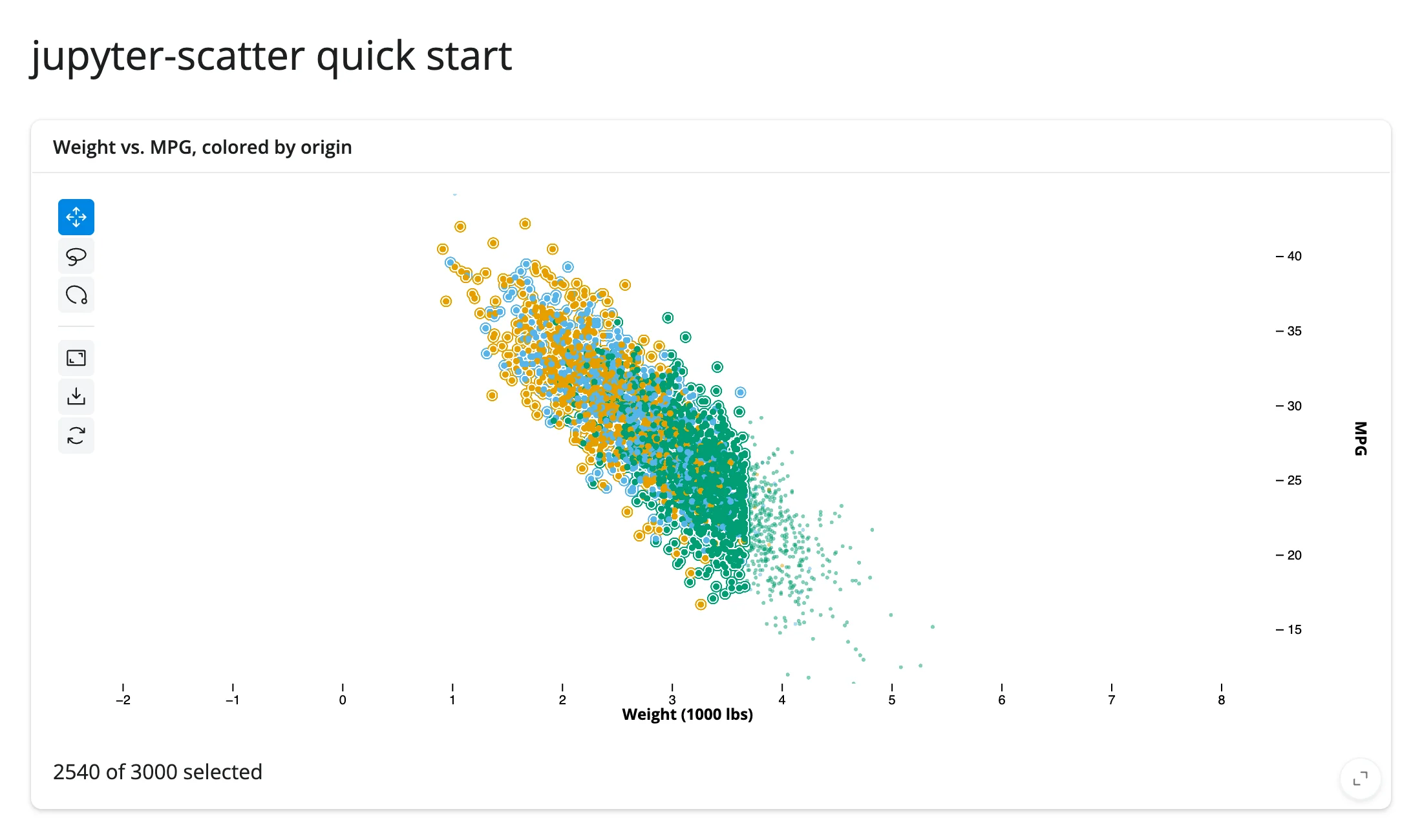
.lasso(initiator=True) lets a user start a lasso with a click-and-drag from anywhere, in addition to the default long-press gesture; both reach plot.selected() the same way. The screenshot above shows the app after lassoing a region: the plot rings the selected points, and the text output below it reads directly off the accessor.
What you can build
Millions of points, interactively
import numpy as np
import pandas as pd
from jscatter import Scatter
from shiny.express import render, ui
from shinywidgets import render_jscatter

N = 2_000_000
rng = np.random.default_rng(0)
centers = rng.uniform(-5, 5, size=(8, 2))
cluster = rng.integers(0, 8, N)
xy = centers[cluster] + rng.normal(scale=0.6, size=(N, 2))
points = pd.DataFrame({"x": xy[:, 0], "y": xy[:, 1], "cluster": cluster.astype(str)})

ui.page_opts(title="2,000,000 points", fillable=True)
ui.p(f"{N:,} points on the GPU. Drag to pan, scroll to zoom, or lasso a cluster.")

with ui.card(full_screen=True):

    @render_jscatter
    def plot():
        return (
            Scatter(data=points, x="x", y="y", color_by="cluster")
            .size(default=2)
            .lasso(initiator=True)
        )

    @render.text
    def n_selected():
        return f"{len(plot.selected()):,} selected"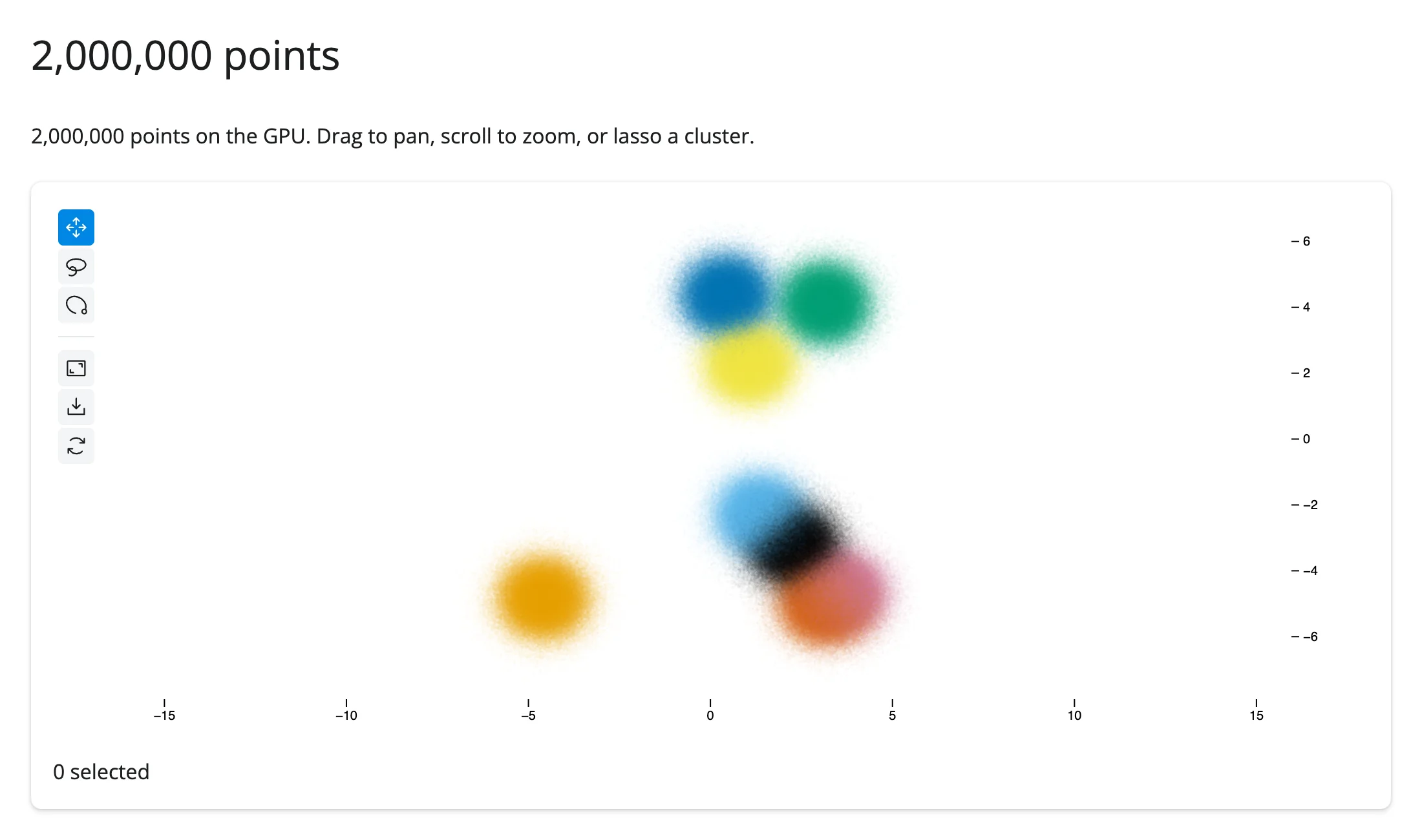
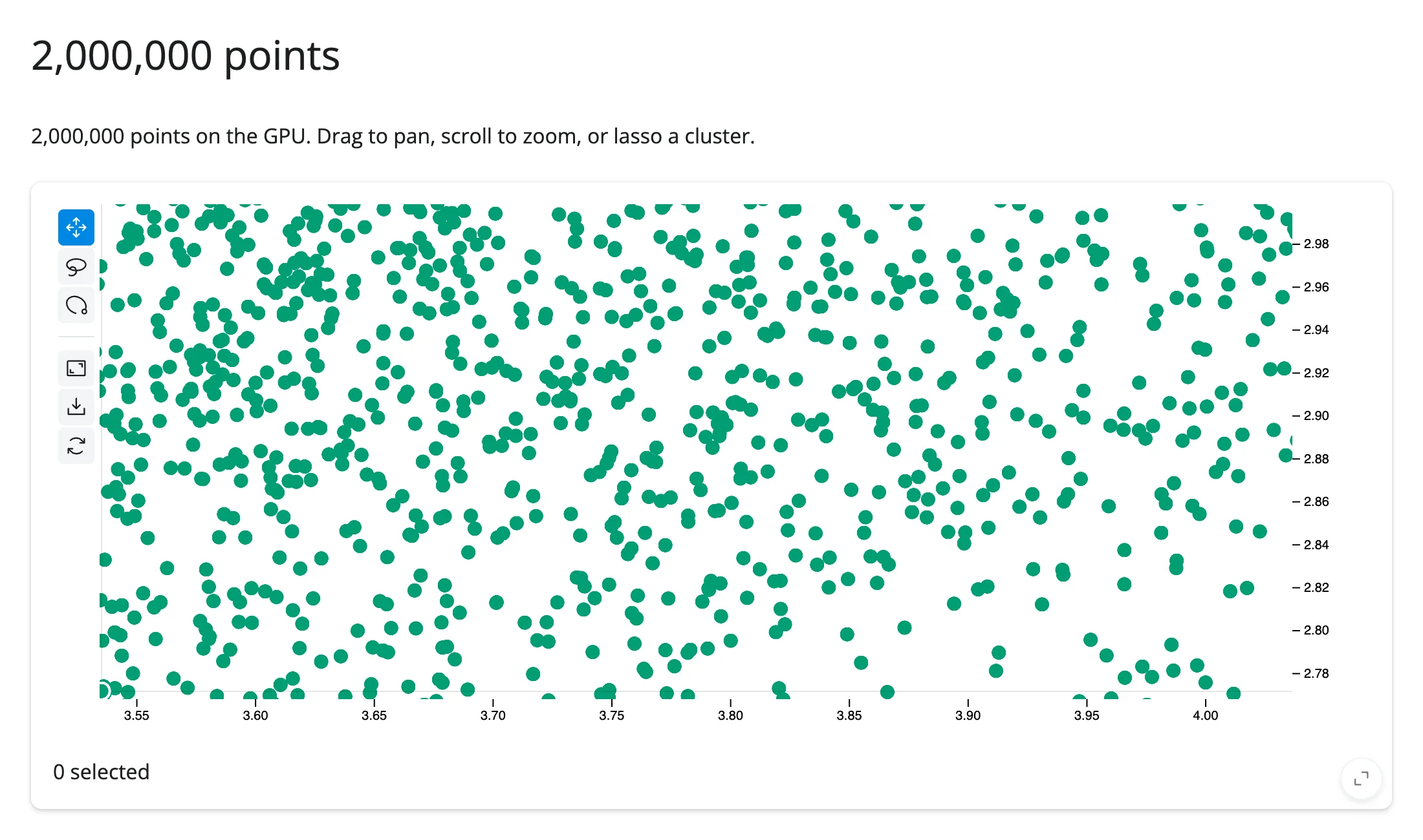
This renders and stays responsive to pan, zoom, and lasso with 2 million points on an ordinary laptop in headless Chromium. Zoomed out, dense clusters blend into soft density blobs (above); scroll in and you see the individual points (below). The practical ceiling is less about rendering and more about getting the selection back to Python – see Gotchas and limitations for the message-size limit on very large lasso selections.
Color, size, and opacity encodings
import numpy as np
import pandas as pd
from jscatter import Scatter
from shiny.express import ui
from shinywidgets import render_jscatter

rng = np.random.default_rng(3)
n = 4000
origin = pd.Series(rng.choice(["USA", "Europe", "Japan"], n, p=[0.5, 0.25, 0.25]))
weight = origin.map({"USA": 3.4, "Europe": 2.6, "Japan": 2.4}) + rng.normal(0, 0.5, n)
cars = pd.DataFrame(
    {
        "origin": origin.astype("category"),
        "weight": weight.round(2),
        "mpg": (45 - 6 * weight + rng.normal(0, 2.5, n)).round(1),
        "hp": (45 * weight + rng.normal(0, 25, n)).round(),
    }
)

ui.page_opts(title="Color, size, and opacity encodings", fillable=True)

with ui.card(full_screen=True):
    ui.card_header("Color = origin, size and opacity = horsepower")

    @render_jscatter
    def plot():
        # jscatter allows at most 2 distinct *data dimensions* driving
        # color/size/opacity at once; reuse one dimension (here "hp") across
        # more than one channel to combine three encodings anyway.
        return (
            Scatter(data=cars, x="weight", y="mpg")
            .color(by="origin")
            .size(by="hp", map=[2, 4, 6, 8, 10])
            .opacity(by="hp")
            .legend(True)
        )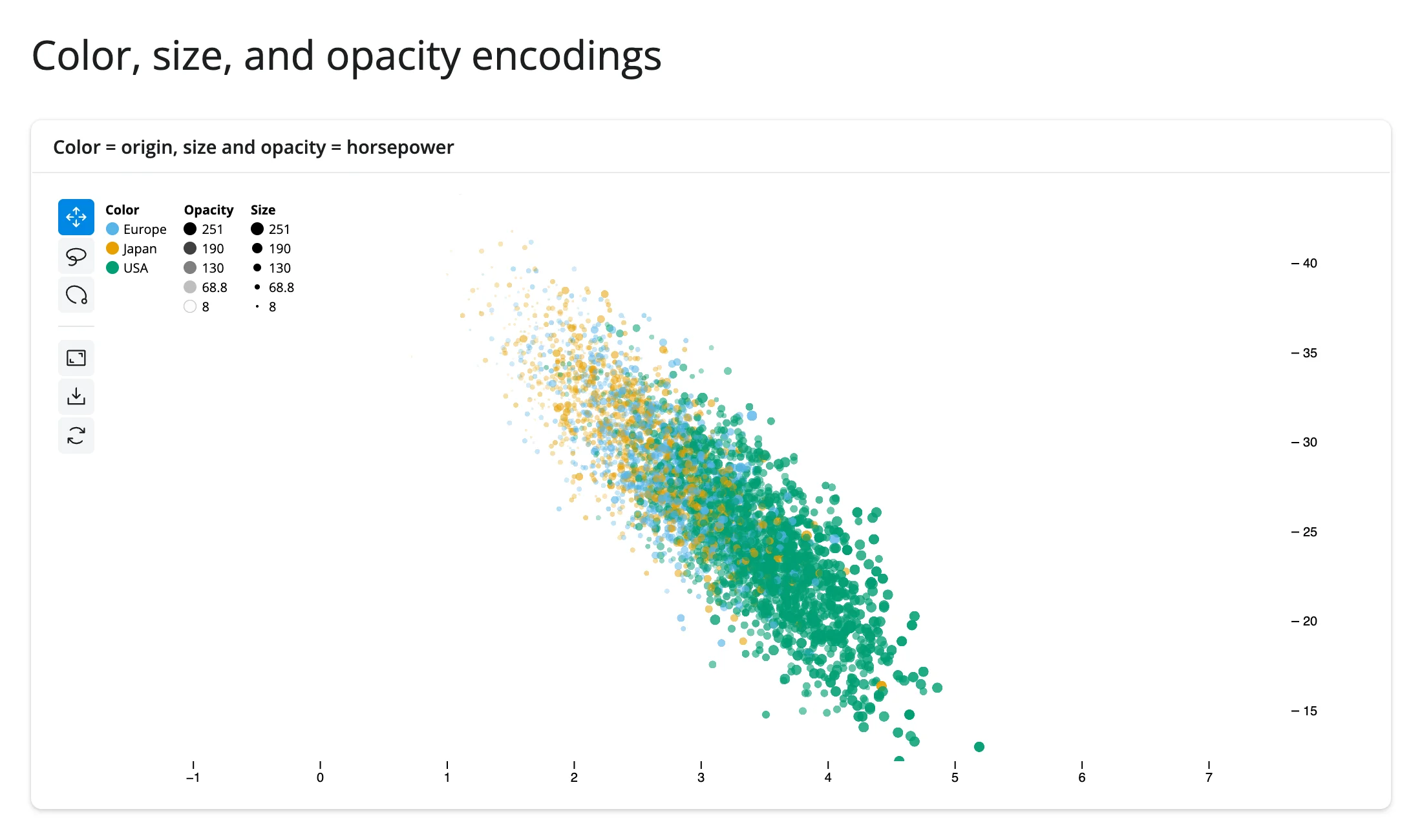
.color(), .size(), and .opacity() all take by= (a column name or array) plus map= for the color/size scale. The legend (.legend(True)) reflects whatever is encoded. One constraint worth knowing before you reach for three encodings: jupyter-scatter packs point attributes into a fixed number of GPU buffer components, so at most 2 distinct data columns can drive color/size/opacity combined – a third distinct column raises AssertionError: Only 2 data encodings are supported. Reusing one column across two channels (as above, hp for both size and opacity) doesn’t count twice.
Animated transitions between embeddings
import numpy as np
import pandas as pd
from jscatter import Scatter
from shiny import reactive
from shiny.express import input, render, ui
from shinywidgets import render_jscatter

rng = np.random.default_rng(2)
n = 600
label = rng.integers(0, 5, n)
grid_x, grid_y = (np.arange(n) % 30).astype(float), (np.arange(n) // 30).astype(float)
angle = rng.uniform(0, 2 * np.pi, n)
radius = label + rng.normal(0, 0.15, n)
points = pd.DataFrame(
    {
        "grid_x": grid_x,
        "grid_y": grid_y,
        "circle_x": radius * np.cos(angle),
        "circle_y": radius * np.sin(angle),
        "label": label.astype(str),
    }
)

ui.page_opts(title="Animated transition between embeddings", fillable=True)
ui.input_action_button("toggle", "Switch embedding", class_="mb-2")

with ui.card(full_screen=True):

    @render_jscatter
    def plot():
        return Scatter(data=points, x="grid_x", y="grid_y", color_by="label")

    @reactive.effect
    @reactive.event(input.toggle)
    def _switch():
        to_circle = input.toggle() % 2 == 1
        x, y = ("circle_x", "circle_y") if to_circle else ("grid_x", "grid_y")
        with reactive.isolate():
            plot.value.xy(x=x, y=y, animate=True)
Before (a grid layout) and after clicking “Switch embedding” (the same points, re-laid-out on a circle, points colored the same throughout):
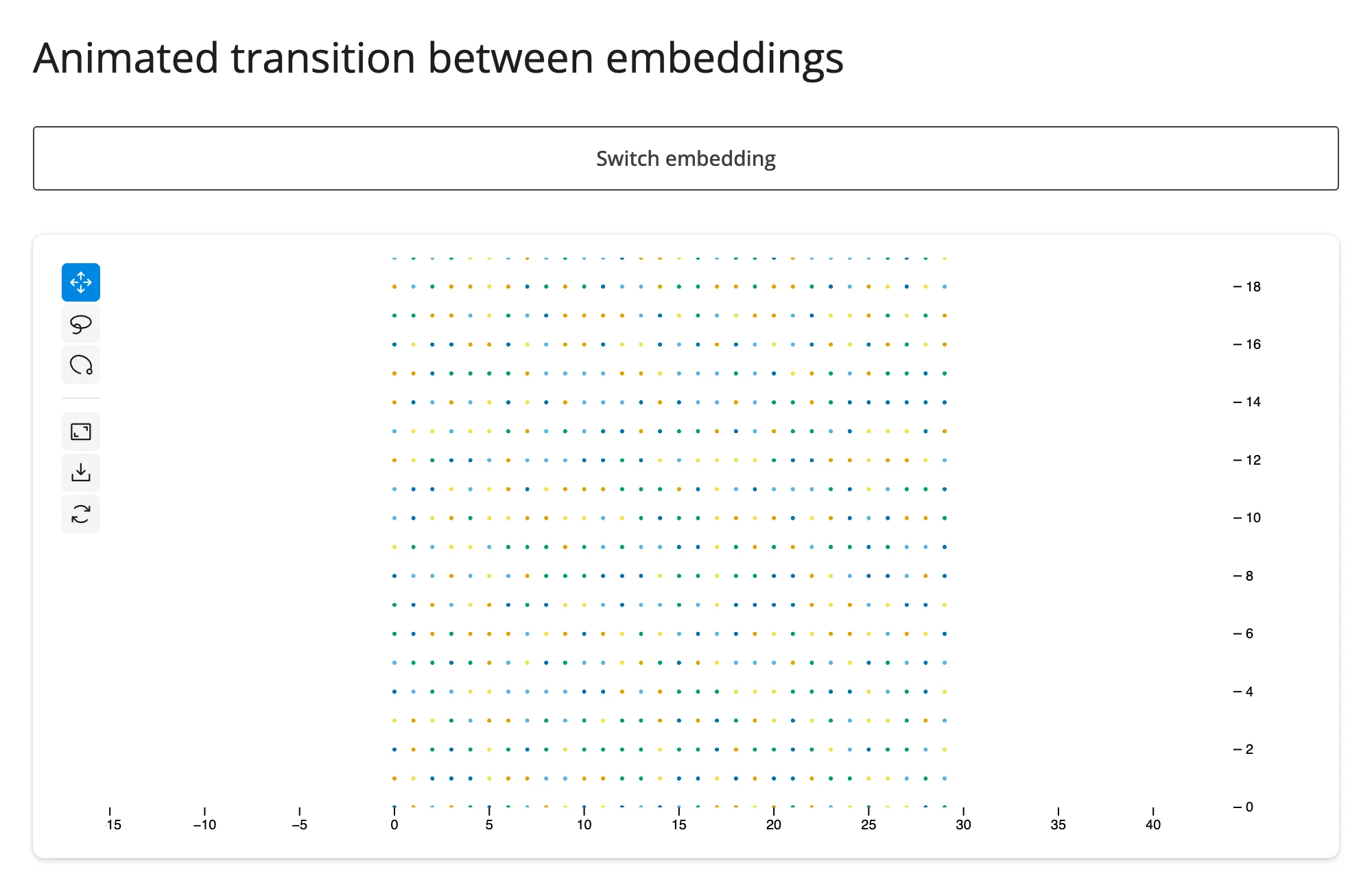
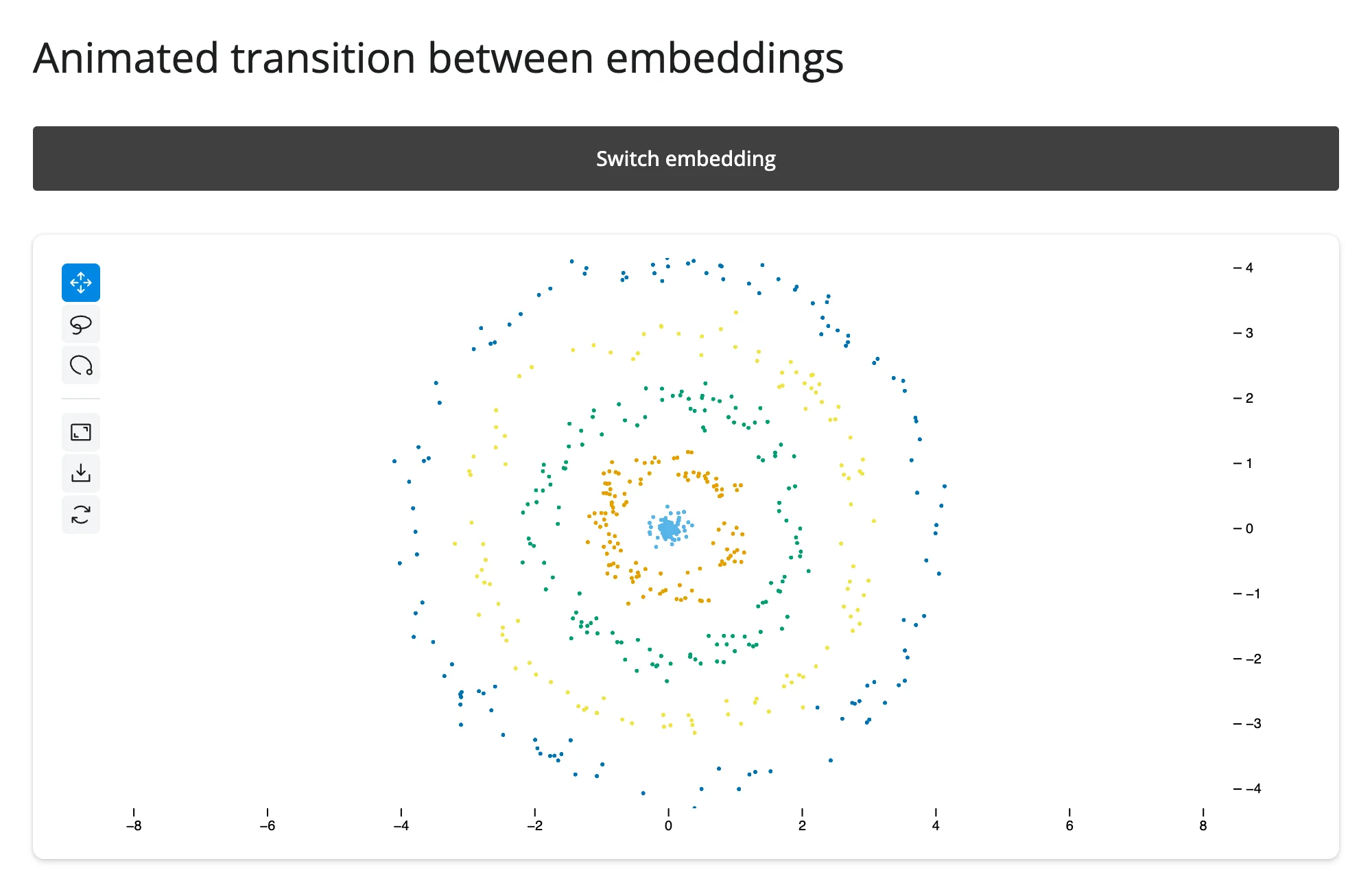
.xy(x=, y=, animate=True) is the one call that moves both coordinates at once and tweens between them – exactly the pattern for comparing two embeddings of the same points (PCA vs. UMAP, before vs. after a model update, raw vs. batch-corrected). It’s called on plot.value (the Scatter builder) inside reactive.isolate(); see Updating the widget from Python for why.
Tooltips with built-in histograms
import numpy as np
import pandas as pd
from jscatter import Scatter
from shiny.express import ui
from shinywidgets import render_jscatter

rng = np.random.default_rng(4)
n = 500
origin = pd.Series(rng.choice(["USA", "Europe", "Japan"], n, p=[0.5, 0.25, 0.25]))
weight = origin.map({"USA": 3.4, "Europe": 2.6, "Japan": 2.4}) + rng.normal(0, 0.5, n)
cars = pd.DataFrame(
    {
        "model": [f"Car {i}" for i in range(n)],
        "origin": origin.astype("category"),
        "weight": weight.round(2),
        "mpg": (45 - 6 * weight + rng.normal(0, 2.5, n)).round(1),
    }
)

ui.page_opts(title="Tooltips", fillable=True)
ui.p("Hover a point to see its data, right in the plot.")

with ui.card(full_screen=True):

    @render_jscatter
    def plot():
        return (
            Scatter(data=cars, x="weight", y="mpg", color_by="origin")
            .tooltip(True, properties=["x", "y", "color", "model"])
        )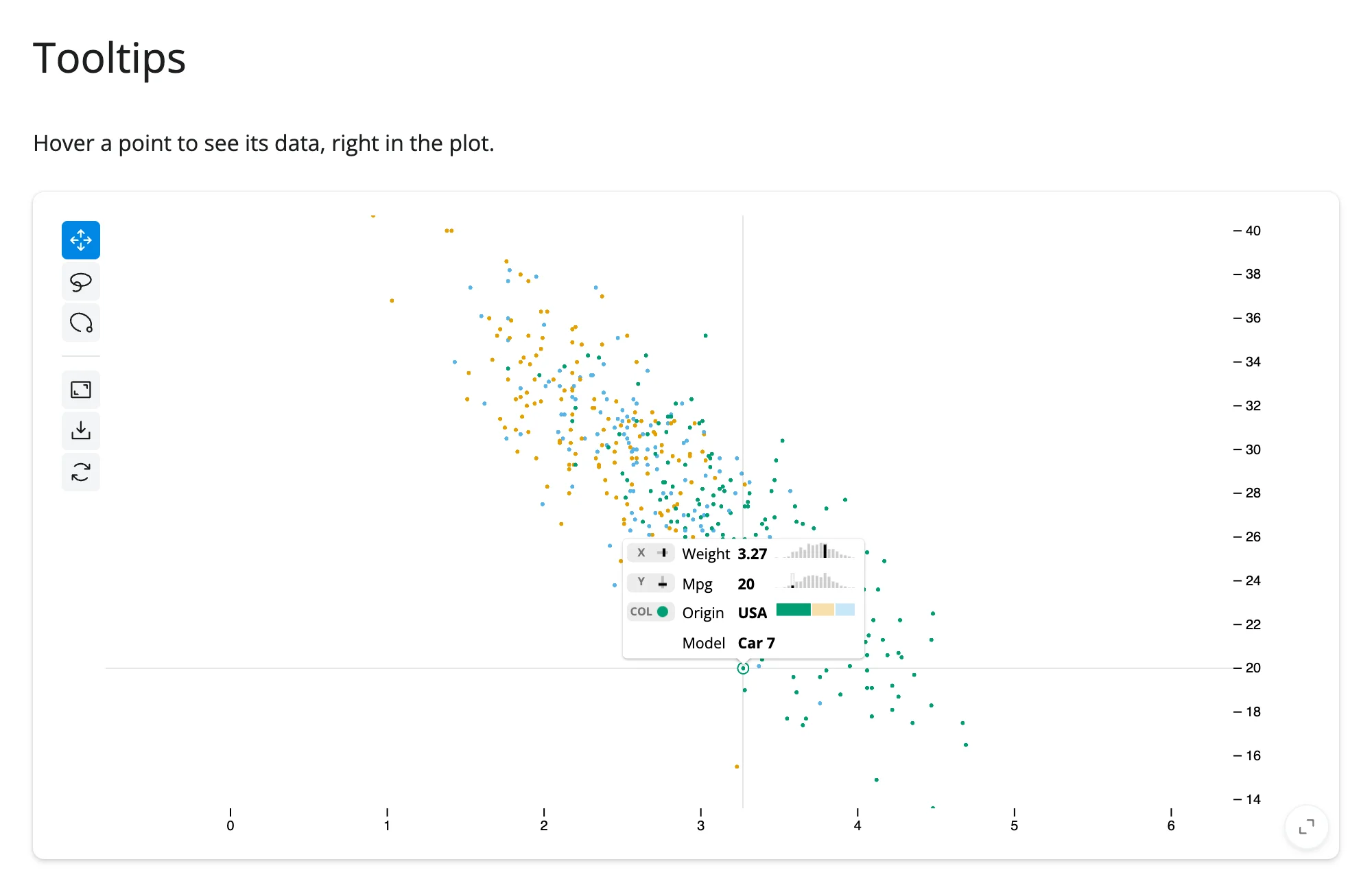
properties names the visual channels ("x", "y", "color", "opacity", "size") that are already encoded, plus any other data column by name ("model" here) – it draws a mini histogram next to each numeric property for free. This is entirely client-side: hovering doesn’t round-trip to Python (see hovering below if you need the hovered point in Python too).
Reacting to user interaction
Accessor reference
| accessor | returns | before any interaction | across re-render | default rate policy |
|---|---|---|---|---|
selected() |
numpy.ndarray (uint32) of row positions |
seeded: empty array (every normal Scatter(...)-returning render); cancels instead, for a bare JupyterScatter built without going through Scatter, until the browser reports once |
re-seeded: a new plot’s selection starts empty | none (reports once per gesture, not during the drag) |
selected_rows(df=None) |
the selected rows of df (default: the frame the Scatter was built with), in df’s own type (pandas, polars, …) |
empty frame (cancels when selected() does) |
derived from selected() |
none (follows selected()) |
selected() cancels the same way reading .widget does before first render – and, only for a bare JupyterScatter constructed without going through Scatter, continues to cancel until the browser reports once. Every normal Scatter(...)-returning render function starts selected() at an empty array immediately instead, since Scatter itself seeds the widget’s selection trait.
selected(): the lasso and click selection, as a reactive value
import numpy as np
import pandas as pd
from jscatter import Scatter
from shiny.express import render, ui
from shinywidgets import render_jscatter

rng = np.random.default_rng(1)
n = 3000
origin = pd.Series(rng.choice(["USA", "Europe", "Japan"], n, p=[0.5, 0.25, 0.25]))
weight = origin.map({"USA": 3.4, "Europe": 2.6, "Japan": 2.4}) + rng.normal(0, 0.5, n)
cars = pd.DataFrame(
    {
        "origin": origin.astype("category"),
        "weight": weight.round(2),
        "mpg": (45 - 6 * weight + rng.normal(0, 2.5, n)).round(1),
    }
)

ui.page_opts(title="plot.selected()", fillable=True)

with ui.layout_columns():
    with ui.card(full_screen=True):

        @render_jscatter
        def plot():
            return Scatter(data=cars, x="weight", y="mpg", color_by="origin").lasso(
                initiator=True
            )

    with ui.card(full_screen=True):

        @render.text
        def n_selected():
            return f"{len(plot.selected())} of {len(cars)} cars selected"

        @render.data_frame
        def selected_cars():
            return plot.selected_rows()
Before any selection, and after lassoing roughly half the plot:
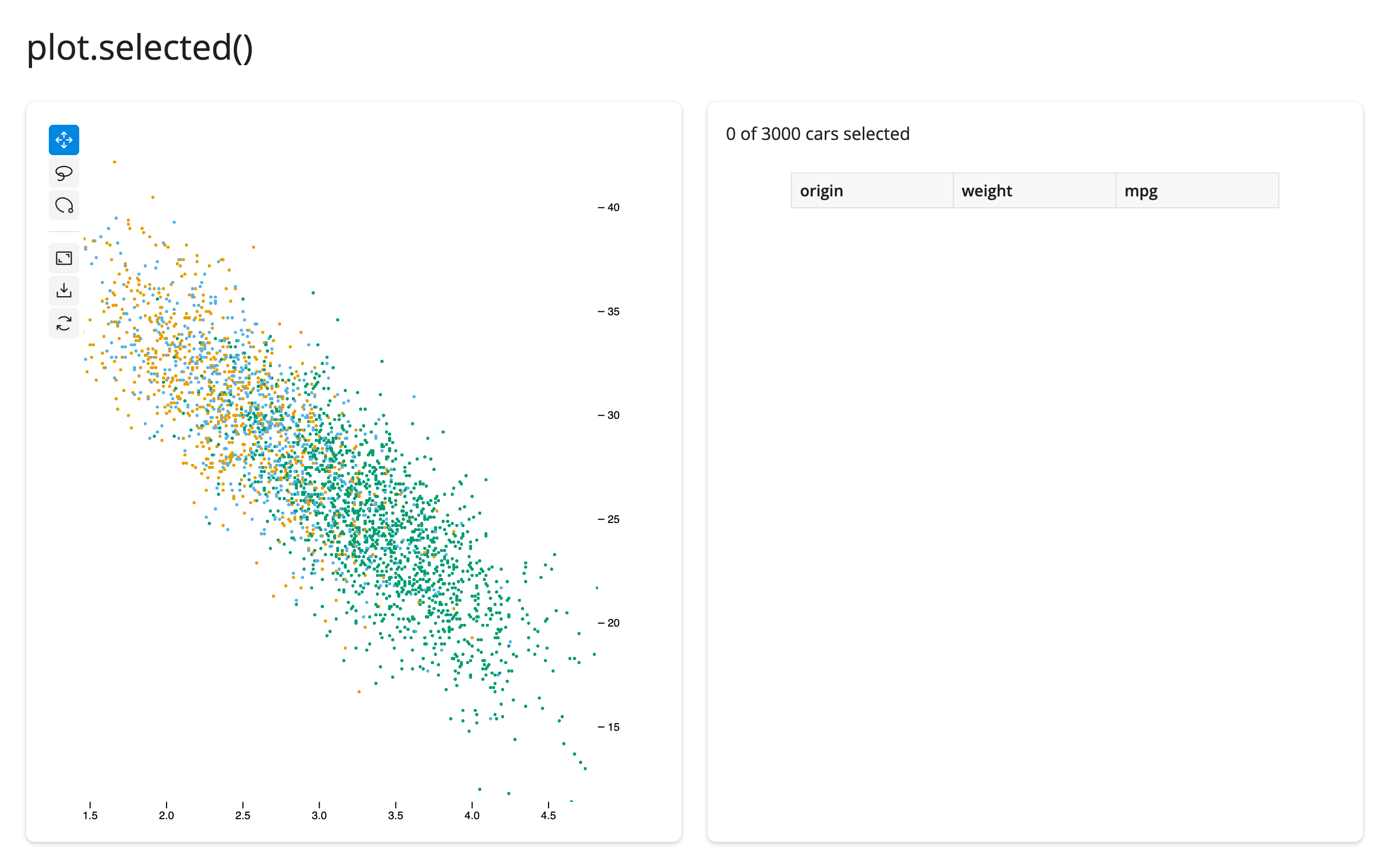
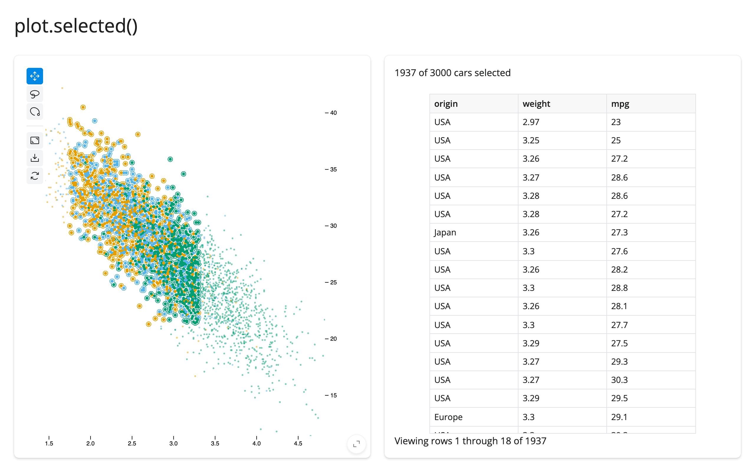
selected() holds row positions into whatever data frame built the plot, not index labels – the right shape for programmatic selection and filtering (see Updating the widget from Python), where the setters also take positions. If you build the plot with Scatter(..., data_use_index=True) and want index labels instead, read plot.value.selection() (the builder’s own method) rather than the accessor. A re-render (e.g., the render function reading an input) gives the user a brand new plot whose selection starts empty; selected() can’t be read inside plot’s own render function for the same reason .widget can’t – read it from another output or a @reactive.effect.
selected_rows(): the selection, as rows of your data frame
When what you want is the selected rows – for a table, a download, or a downstream calculation – plot.selected_rows() is the accessor: it maps the selection’s positions back into the data frame the Scatter was built with and returns those rows (the table in the example above). It’s an empty frame while nothing is selected, so it can be passed straight to @render.data_frame.
Pass a frame explicitly – plot.selected_rows(df) – when the render function returns a bare JupyterScatter (which retains no frame), or when the plot’s rows aren’t your frame’s rows in order. Any frame type works: pandas in, pandas out; polars in, polars out. The match is positional, like df.iloc[plot.selected()] – after a re-render or in-place data replacement with different rows, a retained position can point at a different row, so carry an ID column and look rows up by it when the data can change.
Beyond the accessor: .read()
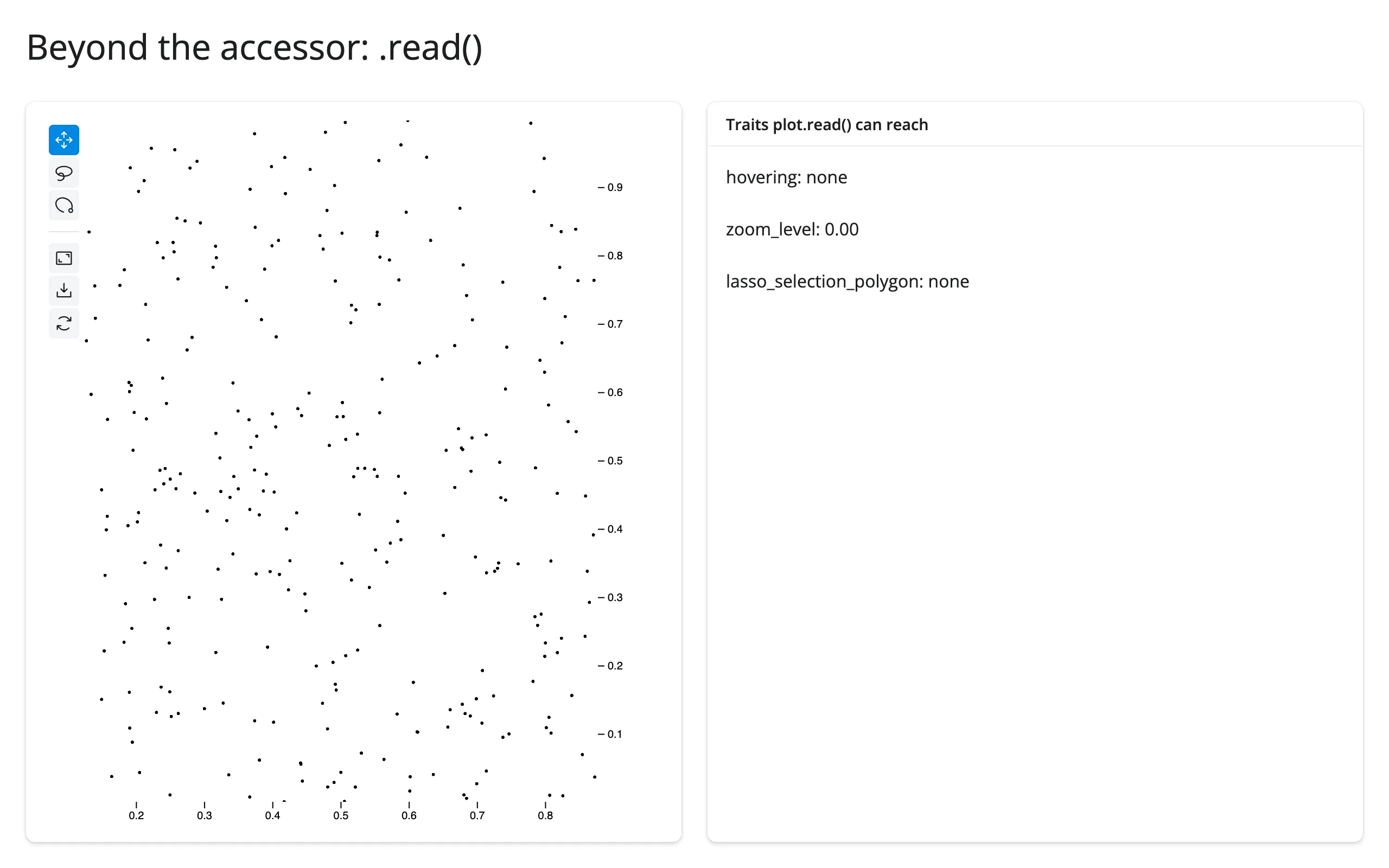
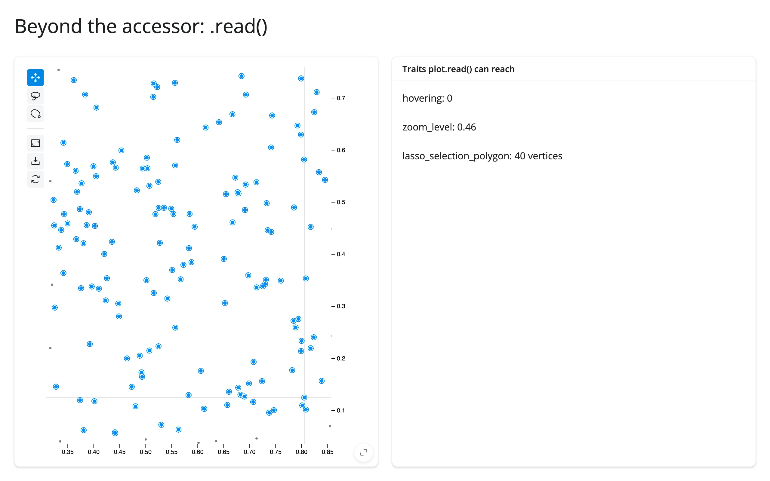
hovering, zoom_level, and lasso_selection_polygon are synced traits of the plot’s own widget, with no dedicated accessor. Because they’re traits of the output’s own widget (not a nested object), plot.read(name) reaches them directly – no reactive_read(), and no req(plot.widget) guard to write yourself; .read() cancels on its own until the plot first renders, the same way the selected() accessor does.
import numpy as np
import pandas as pd
from jscatter import Scatter
from shiny.express import render, ui
from shinywidgets import render_jscatter

rng = np.random.default_rng(5)
n = 400
points = pd.DataFrame({"x": rng.uniform(0, 1, n), "y": rng.uniform(0, 1, n)})

ui.page_opts(title="Beyond the accessor: .read()", fillable=True)

with ui.layout_columns():
    with ui.card(full_screen=True):

        @render_jscatter
        def plot():
            return Scatter(data=points, x="x", y="y").lasso(initiator=True)

    with ui.card():
        ui.card_header("Traits plot.read() can reach")

        @render.text
        def hovering():
            idx = plot.read("hovering")
            return f"hovering: {'none' if idx is None else idx}"

        @render.text
        def zoom_level():
            return f"zoom_level: {plot.read('zoom_level'):.2f}"

        @render.text
        def lasso_polygon():
            poly = plot.read("lasso_selection_polygon")
            return f"lasso_selection_polygon: {'none' if poly is None else f'{len(poly)} vertices'}"
Before interacting, and after hovering a point, scroll-zooming, and lassoing (all three traits update):
Three widget traits are worth reading this way beyond the selected() accessor:
hovering: the row position under the cursor, orNone. Updates on every mouse move over a point – don’t feed it straight into an expensive computation without debouncing.zoom_level: a read-only float that tracks the camera’s zoom factor, updated on every scroll/pan.lasso_selection_polygon: the lasso’s own vertices in data coordinates (an(n, 2)array),Noneuntil the first lasso. Useful if you want the shape of the selection rather than just which points it contains (e.g., to draw the same region on a second, differently-scaled plot).
filter is also a synced trait, but nothing in jupyter-scatter’s UI writes to it; it’s Python-to-browser only (see Programmatic selection and filtering), so there’s no browser gesture to read it for.
Rate limiting
jupyter-scatter reports selection once when a gesture ends, not continuously during the drag, so render_jscatter’s selected() has no default rate policy – there’s nothing streaming to coalesce. If you share one plot across many sessions (a process-global or shared_lifetime() widget) and several sessions react to the same selection with expensive work, pass rate_policy="debounce" and rate_delay= to @render_jscatter(...), the same two keyword arguments every renderer in this roster accepts. There’s no jscatter-specific tuning beyond deciding whether you need this at all.
Reading an accessor on demand
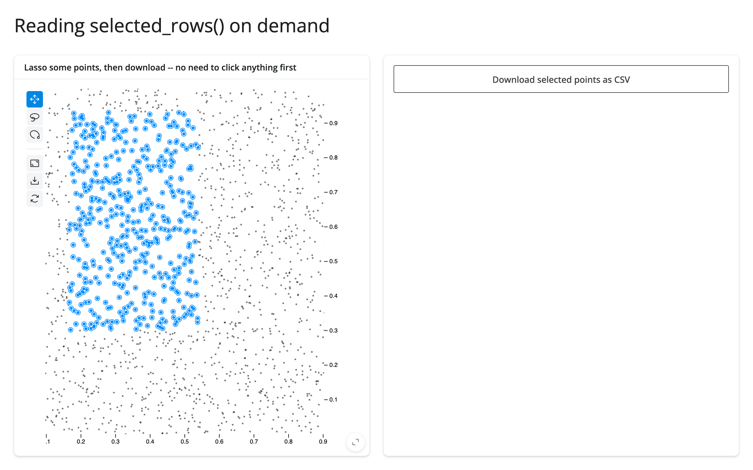
selected_rows() is seeded empty the moment a Scatter(...)-built plot renders, so it’s safe to read from somewhere that only runs occasionally – a download handler, say – with no prior interaction needed first:
import numpy as np
import pandas as pd
from jscatter import Scatter
from shiny.express import render, ui
from shinywidgets import render_jscatter

rng = np.random.default_rng(1)
n = 2000
points = pd.DataFrame({"x": rng.uniform(0, 1, n), "y": rng.uniform(0, 1, n)})

ui.page_opts(title="Reading selected_rows() on demand", fillable=True)

with ui.layout_columns():
    with ui.card(full_screen=True):
        ui.card_header("Lasso some points, then download -- no need to click anything first")

        @render_jscatter
        def plot():
            return Scatter(data=points, x="x", y="y").lasso(initiator=True)

    with ui.card():

        @render.download_button(
            filename="selected.csv", label="Download selected points as CSV"
        )
        def download():
            # selected_rows() is seeded empty the moment the plot renders, so
            # this reads whatever's currently selected, even on first run.
            yield plot.selected_rows().to_csv(index=False)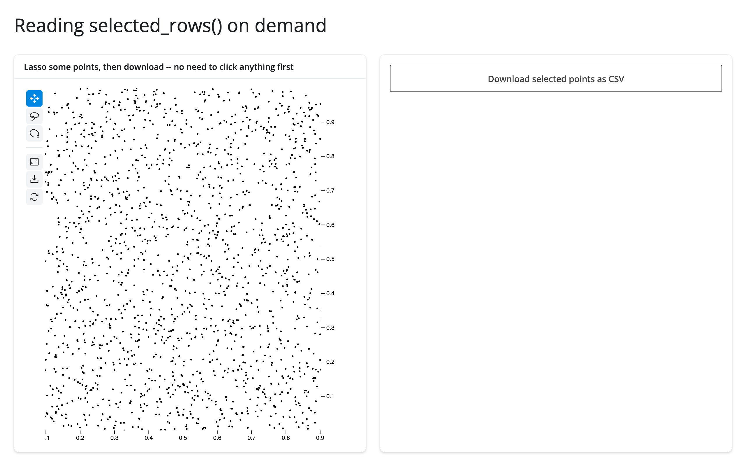
Updating the widget from Python
Two ways to change an already-rendered plot, and when each is right:
- Re-render (have the render function return a new
Scatter): simplest, but jupyter-scatter re-sends the full point data and the view resets – camera, zoom, and selection are all lost. Fine for small data or when the whole plot is genuinely changing (e.g., a different data frame entirely). - Update in place, from a
@reactive.effect, reading the input that should drive the change and calling a method onplot.value(theScatterbuilder) or setting a trait directly onplot.widget, both wrapped inreactive.isolate()so reading the current state of the plot doesn’t create a reactive dependency that would re-run the effect in a loop. This is almost always what you want for anything short of swapping the dataset: the camera, zoom, and selection are preserved, and jupyter-scatter’s ~2 MB JS bundle and the point data aren’t re-sent.
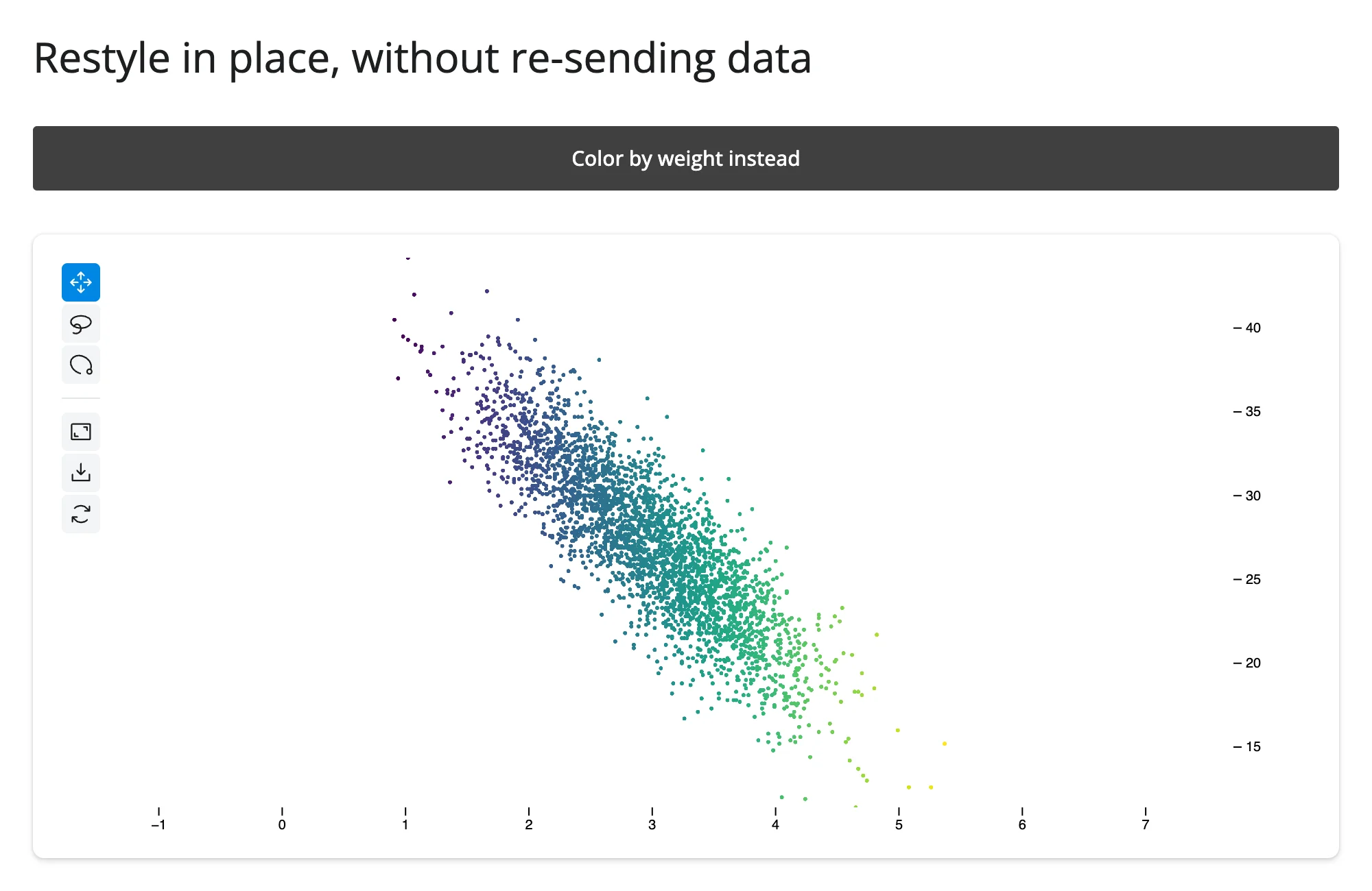
examples/08_update_in_place.py shows the .value form, recoloring a plot from categorical to continuous on a button click without re-rendering or losing the current view:
import numpy as np
import pandas as pd
from jscatter import Scatter
from shiny import reactive
from shiny.express import input, render, ui
from shinywidgets import render_jscatter

rng = np.random.default_rng(1)
n = 3000
origin = pd.Series(rng.choice(["USA", "Europe", "Japan"], n, p=[0.5, 0.25, 0.25]))
weight = origin.map({"USA": 3.4, "Europe": 2.6, "Japan": 2.4}) + rng.normal(0, 0.5, n)
cars = pd.DataFrame({"origin": origin.astype("category"), "weight": weight.round(2)})
cars["mpg"] = (45 - 6 * cars["weight"] + rng.normal(0, 2.5, n)).round(1)

ui.page_opts(title="Restyle in place, without re-sending data", fillable=True)
ui.input_action_button("toggle", "Color by weight instead", class_="mb-2")

with ui.card(full_screen=True):

    @render_jscatter
    def plot():
        return Scatter(data=cars, x="weight", y="mpg", color_by="origin")

    @reactive.effect
    @reactive.event(input.toggle)
    def _recolor():
        by_weight = input.toggle() % 2 == 1
        with reactive.isolate():
            if by_weight:
                plot.value.color(by="weight", map="viridis")
            else:
                plot.value.color(by="origin")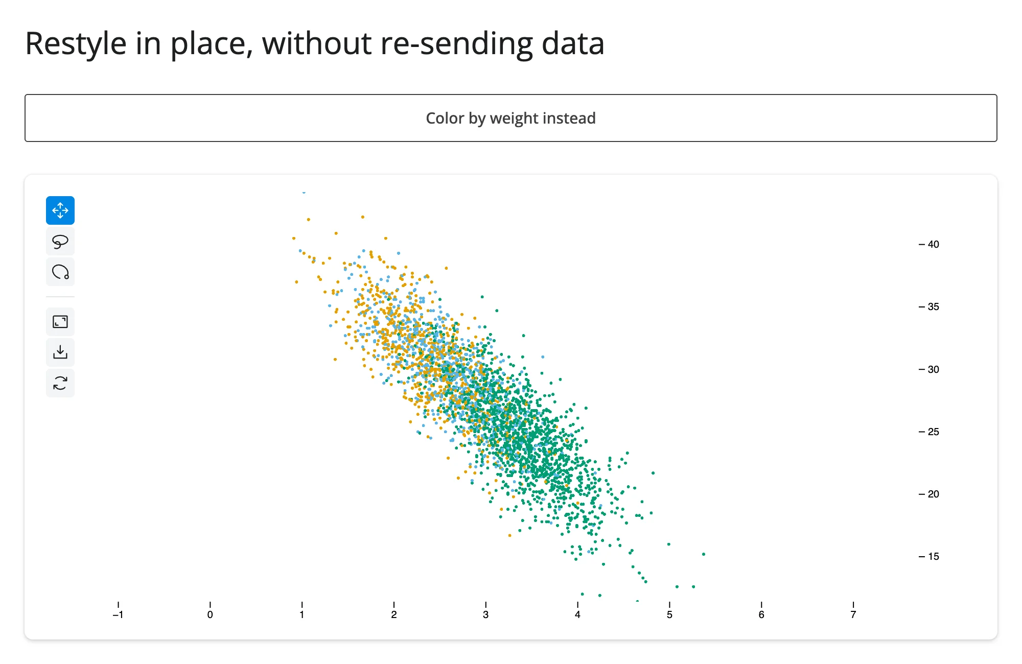
Programmatic selection and filtering from Python
examples/09_python_selection_filter.py drives both selection and filter straight from Python, by assigning the widget’s traits directly (the form the class docstring recommends) rather than chaining Scatter methods:
import numpy as np
import pandas as pd
from jscatter import Scatter
from shiny import reactive
from shiny.express import input, render, ui
from shinywidgets import render_jscatter

rng = np.random.default_rng(1)
n = 3000
origin = pd.Series(rng.choice(["USA", "Europe", "Japan"], n, p=[0.5, 0.25, 0.25]))
weight = origin.map({"USA": 3.4, "Europe": 2.6, "Japan": 2.4}) + rng.normal(0, 0.5, n)
cars = pd.DataFrame({"origin": origin.astype("category"), "weight": weight.round(2)})
cars["mpg"] = (45 - 6 * cars["weight"] + rng.normal(0, 2.5, n)).round(1)

ui.page_opts(title="Drive selection and filter from Python", fillable=True)
with ui.layout_columns(col_widths=[4, 4, 4]):
    ui.input_action_button("select_heavy", "Select heaviest 10%")
    ui.input_action_button("filter_usa", "Filter to USA only")
    ui.input_action_button("reset", "Reset")

with ui.card(full_screen=True):

    @render_jscatter
    def plot():
        return Scatter(data=cars, x="weight", y="mpg", color_by="origin")

    @reactive.effect
    @reactive.event(input.select_heavy)
    def _select():
        cutoff = cars["weight"].quantile(0.9)
        ids = np.flatnonzero(cars["weight"] >= cutoff).astype("uint32")
        with reactive.isolate():
            plot.widget.selection = ids

    @reactive.effect
    @reactive.event(input.filter_usa)
    def _filter():
        ids = np.flatnonzero(cars["origin"] == "USA").astype("uint32")
        with reactive.isolate():
            plot.widget.filter = ids

    @reactive.effect
    @reactive.event(input.reset)
    def _reset():
        with reactive.isolate():
            plot.widget.selection = np.array([], dtype="uint32")
            plot.widget.filter = None

    @render.text
    def n_selected():
        return f"{len(plot.selected()):,} selected"
After “Select heaviest 10%” (selection rings the selected points; the rest of the data stays visible), and after “Filter to USA only” (filtering actually hides the other points, rather than just marking them):
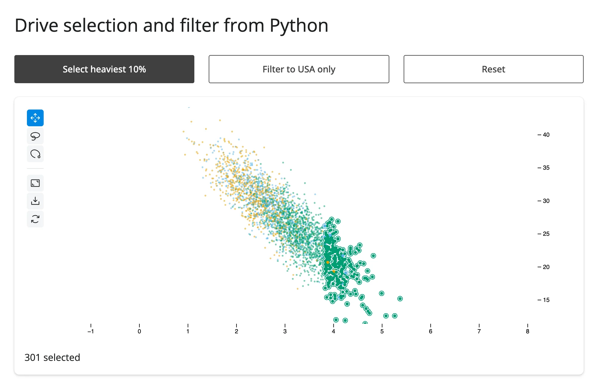
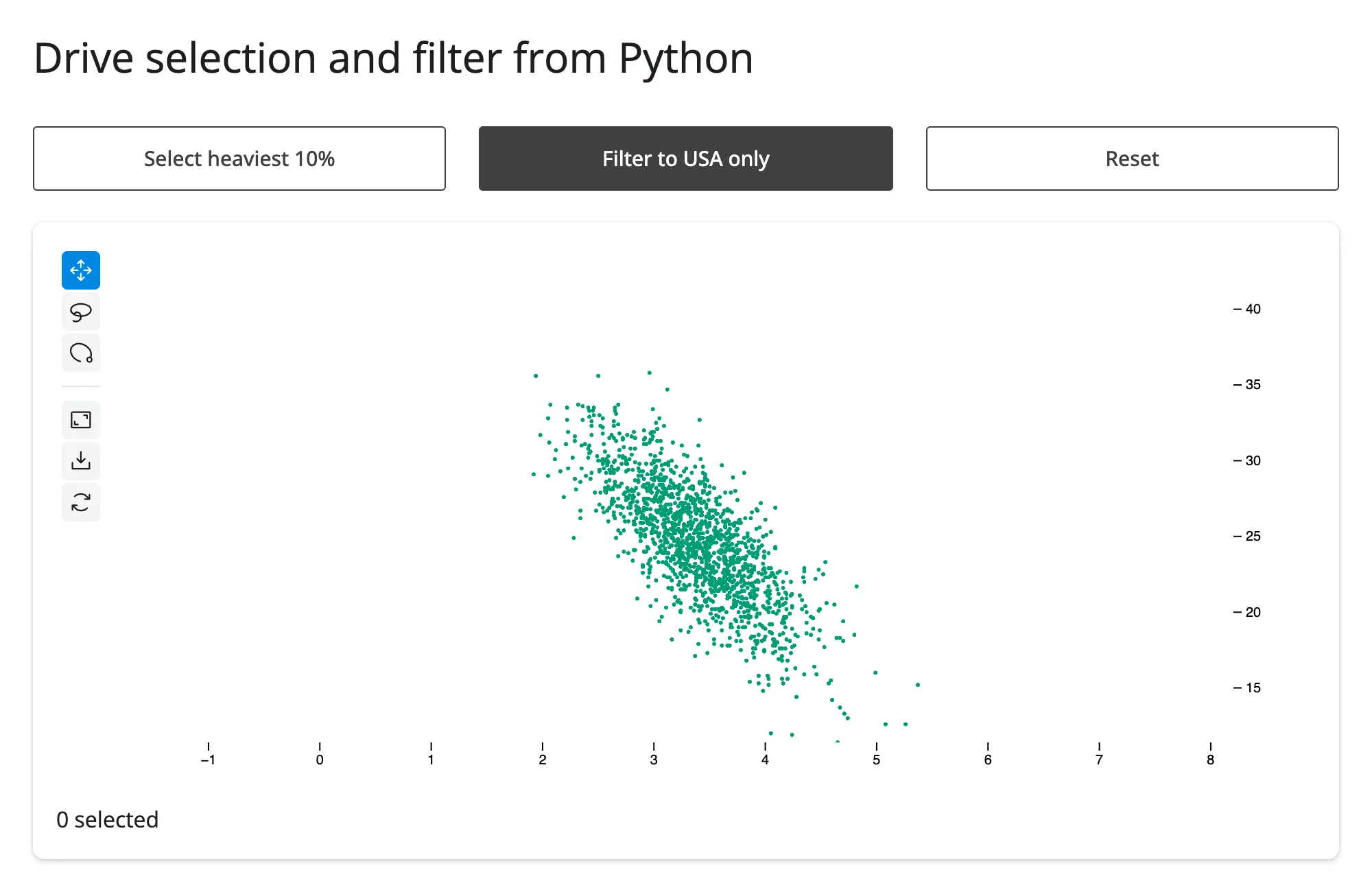
selection highlights points without hiding anything else; filter hides everything not in the given set of positions. Both take uint32 arrays of row positions (or index labels if the Scatter was built with data_use_index=True); set either to None (filter) or an empty array (selection) to clear it. Both also have chainable equivalents on the Scatter builder (plot.value.selection(ids), plot.value.filter(ids)) if you’re already calling other builder methods in the same effect.
Coordinating multiple views
Linked brushing between two jscatter plots
examples/10_linked_brushing.py mirrors each plot’s lasso selection onto the other, so selecting the same underlying rows highlights consistently regardless of which plot the user dragged on:
import numpy as np
import pandas as pd
from jscatter import Scatter
from shiny import reactive
from shiny.express import ui
from shinywidgets import render_jscatter

rng = np.random.default_rng(1)
n = 3000
origin = pd.Series(rng.choice(["USA", "Europe", "Japan"], n, p=[0.5, 0.25, 0.25]))
weight = origin.map({"USA": 3.4, "Europe": 2.6, "Japan": 2.4}) + rng.normal(0, 0.5, n)
cars = pd.DataFrame({"origin": origin.astype("category"), "weight": weight.round(2)})
cars["mpg"] = (45 - 6 * cars["weight"] + rng.normal(0, 2.5, n)).round(1)
cars["hp"] = (45 * cars["weight"] + rng.normal(0, 25, n)).round()

ui.page_opts(title="Linked brushing between two jscatter plots", fillable=True)

with ui.layout_columns():
    with ui.card(full_screen=True):
        ui.card_header("Weight vs. MPG")

        @render_jscatter
        def weight_mpg():
            return Scatter(data=cars, x="weight", y="mpg", color_by="origin").lasso(
                initiator=True
            )

    with ui.card(full_screen=True):
        ui.card_header("Horsepower vs. MPG")

        @render_jscatter
        def hp_mpg():
            return Scatter(data=cars, x="hp", y="mpg", color_by="origin").lasso(
                initiator=True
            )


def link(source, target):
    @reactive.effect
    def _():
        selection = source.selected()
        with reactive.isolate():
            if not np.array_equal(selection, target.widget.selection):
                target.widget.selection = selection


link(weight_mpg, hp_mpg)
link(hp_mpg, weight_mpg)
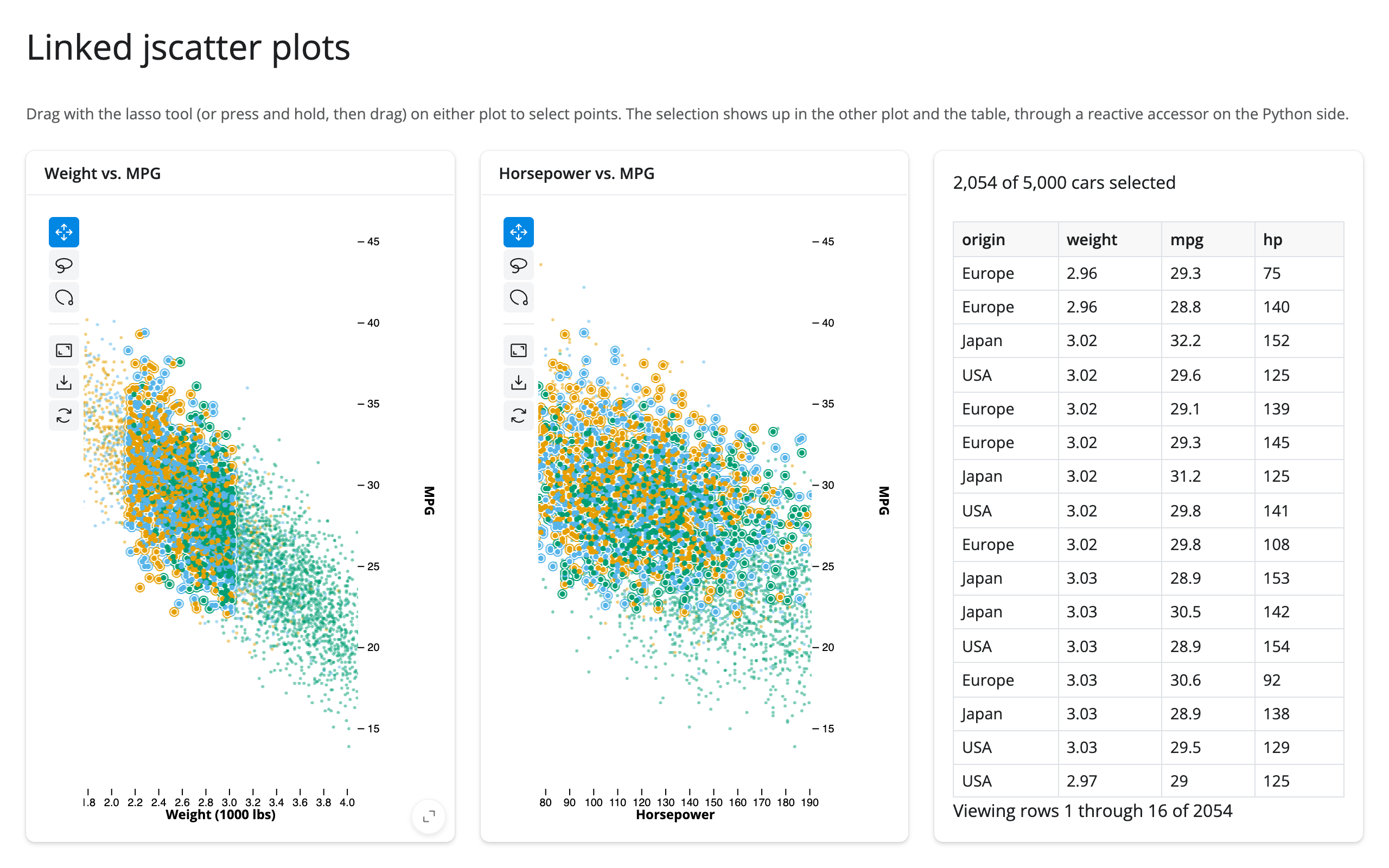
Before, and after lassoing the lighter half of the weight/MPG plot (the same cars light up in the horsepower plot, which has its own, uncorrelated noise):
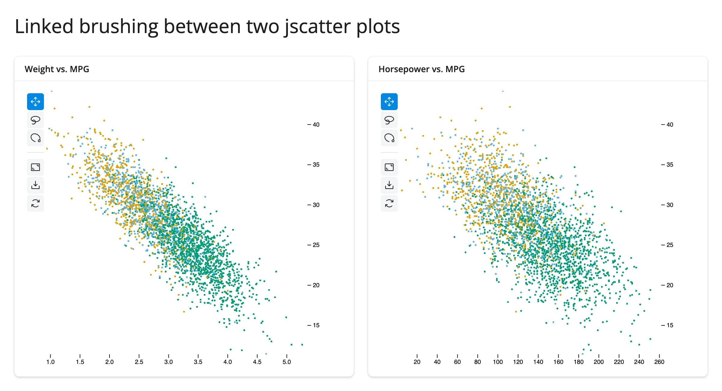
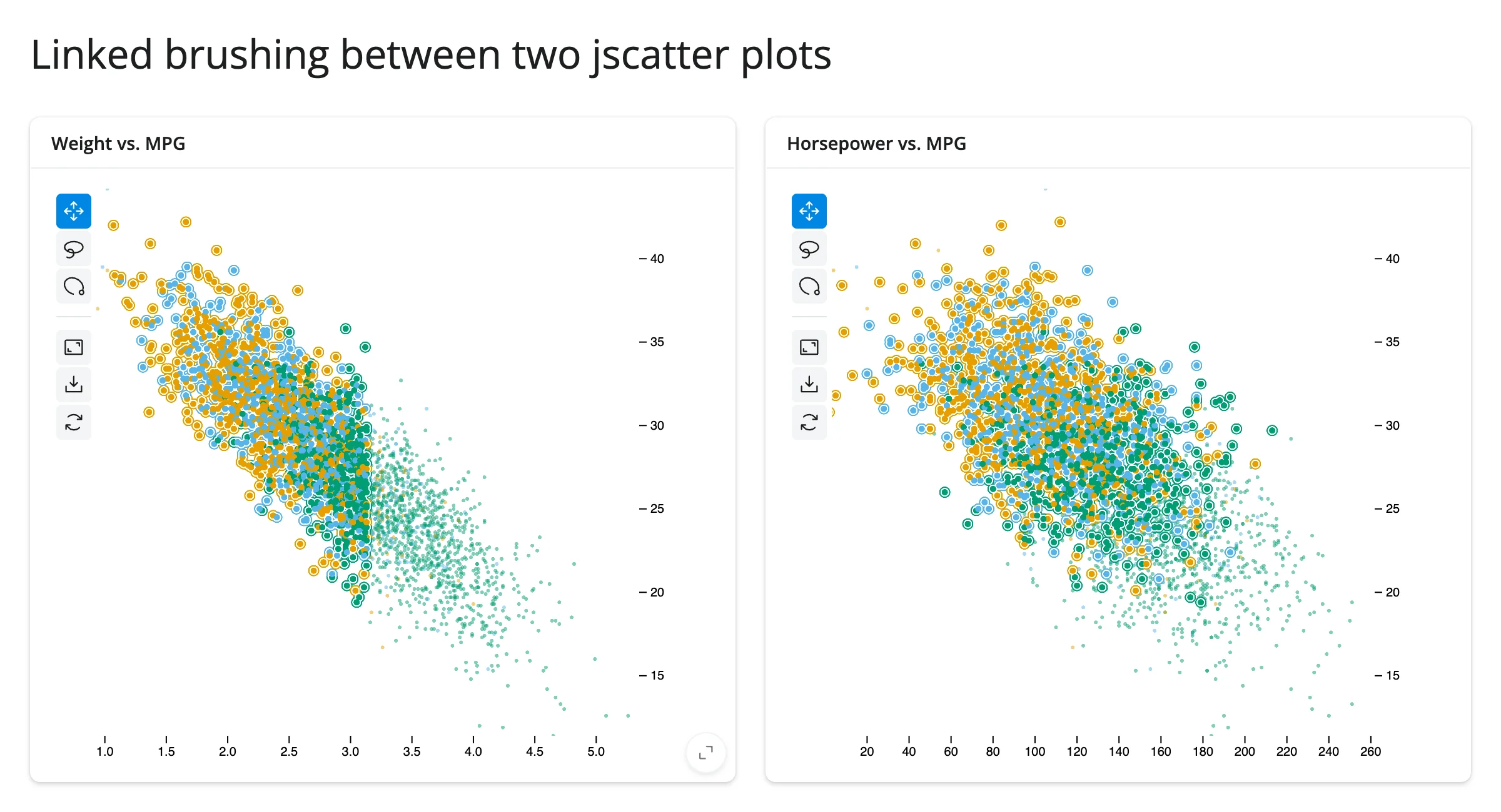
The np.array_equal guard is load-bearing: without it, each plot setting the other’s selection would trigger the other effect right back, which (even though it converges) does unnecessary work on every gesture.
Lasso selection drives a table in another widget
examples/11_lasso_to_itables.py feeds selected_rows() into an itables table, re-rendered to show only the lassoed rows – a different widget library entirely, linked with one line of Python:
import numpy as np
import pandas as pd
from jscatter import Scatter
from shiny.express import ui
from shinywidgets import render_itables, render_jscatter

rng = np.random.default_rng(1)
n = 1500
origin = pd.Series(rng.choice(["USA", "Europe", "Japan"], n, p=[0.5, 0.25, 0.25]))
weight = origin.map({"USA": 3.4, "Europe": 2.6, "Japan": 2.4}) + rng.normal(0, 0.5, n)
cars = pd.DataFrame({"origin": origin.astype("category"), "weight": weight.round(2)})
cars["mpg"] = (45 - 6 * cars["weight"] + rng.normal(0, 2.5, n)).round(1)

ui.page_opts(title="Lasso selection drives an itables table", fillable=True)

with ui.layout_columns():
    with ui.card(full_screen=True):

        @render_jscatter
        def plot():
            return Scatter(data=cars, x="weight", y="mpg", color_by="origin").lasso(
                initiator=True
            )

    with ui.card(full_screen=True):
        ui.card_header("Rows inside the lasso")

        @render_itables
        def table():
            return plot.selected_rows()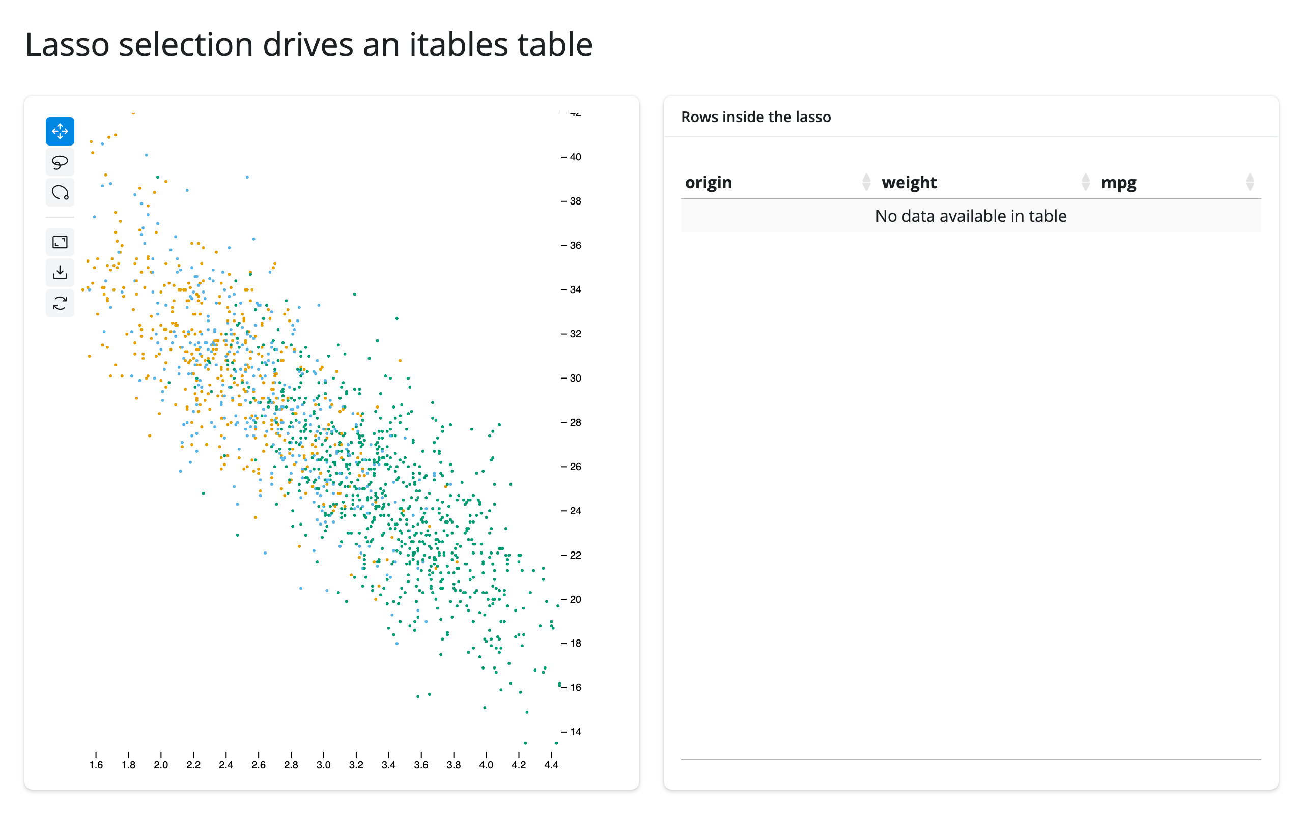
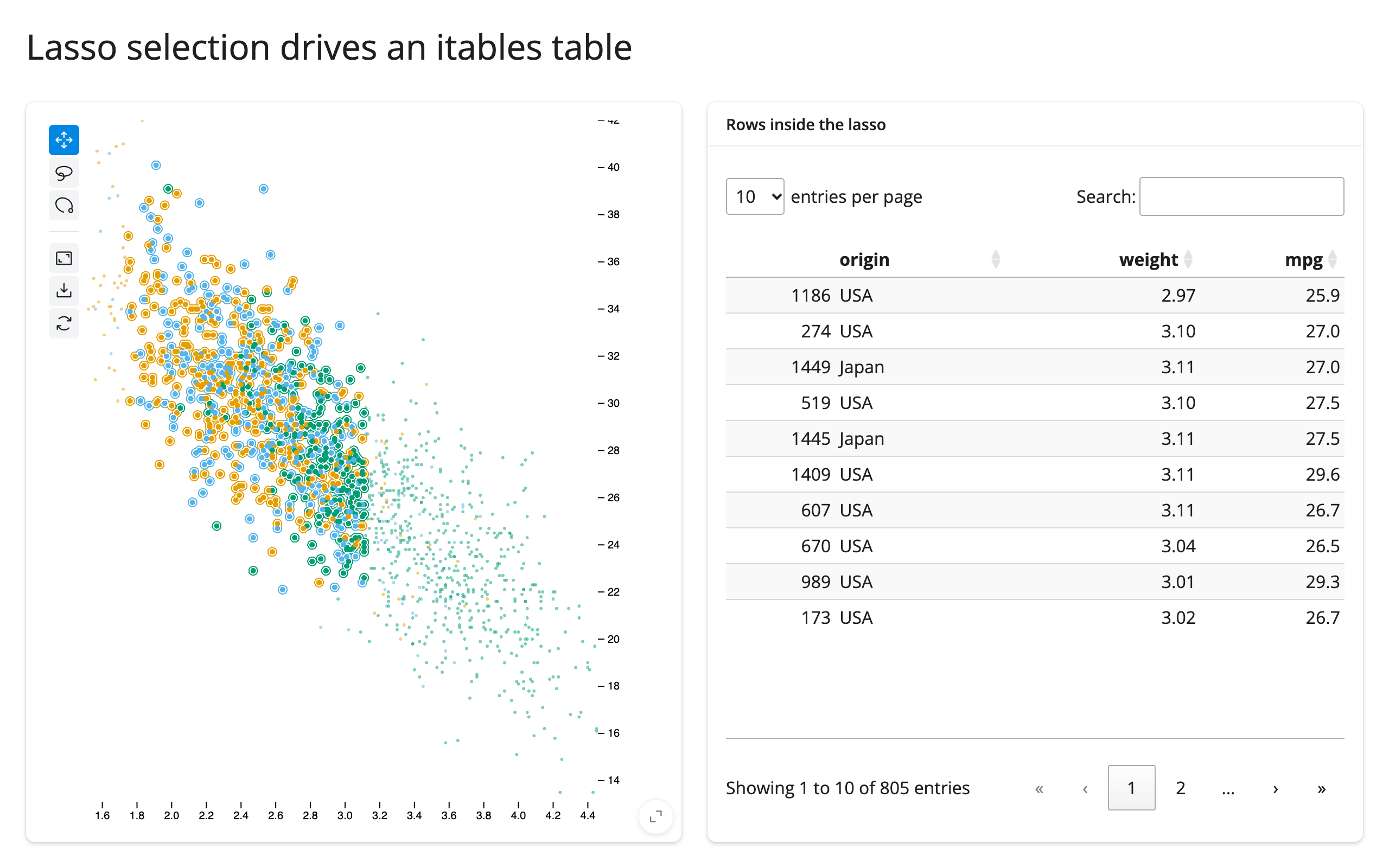
This re-renders the table on every selection change rather than updating it in place – simple, and cheap enough for tables up to a few tens of thousands of rows. For a table that’s expensive to rebuild, read plot.selected_rows() in an effect and call .widget.update(...) (see the itables guide) instead.
Table row selection highlights the plot
The same link, run the other way: examples/12_table_to_plot_highlight.py uses Shiny’s own @render.data_frame row selection to highlight matching points in a jscatter plot.
import numpy as np
import pandas as pd
from jscatter import Scatter
from shiny import reactive, req
from shiny.express import render, ui
from shinywidgets import render_jscatter

rng = np.random.default_rng(6)
cars = pd.DataFrame(
    {
        "model": [f"Car {i}" for i in range(60)],
        "weight": rng.uniform(1.8, 4.5, 60).round(2),
        "mpg": rng.uniform(14, 44, 60).round(1),
    }
)

ui.page_opts(title="Table row selection highlights the plot", fillable=True)

with ui.layout_columns():
    with ui.card(full_screen=True):

        @render.data_frame
        def table():
            return render.DataGrid(cars, selection_mode="rows")

    with ui.card(full_screen=True):

        @render_jscatter
        def plot():
            return Scatter(data=cars, x="weight", y="mpg")

        @reactive.effect
        def _highlight():
            rows = table.cell_selection()["rows"]
            w = plot.widget
            req(w)
            ids = np.array(rows, dtype="uint32")
            with reactive.isolate():
                w.selection = ids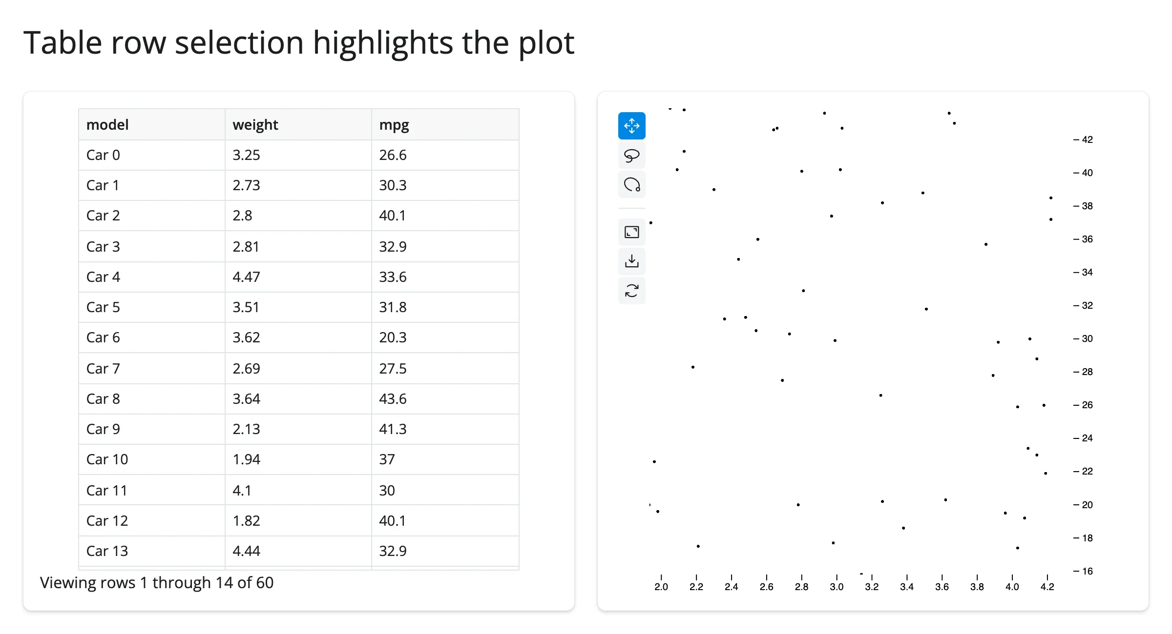
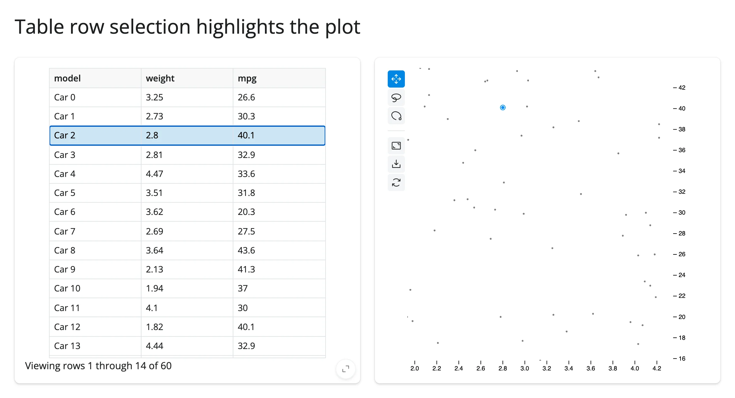
table.cell_selection()["rows"] gives row positions in the table’s own display order; since this example builds both the table and the plot from the identical, unsorted cars frame, those positions line up directly with plot.widget.selection’s row positions. If your table can be sorted or filtered, map through the visible-row positions first (see the ipydatagrid or itables guides).
Large data
jupyter-scatter’s whole premise is scale: every point is drawn by the GPU (via regl-scatterplot) instead of the DOM, so there’s no separate “large data mode” to opt into – see Millions of points, interactively above, which renders and stays responsive to pan, zoom, and lasso with 2,000,000 points. The practical ceiling isn’t rendering, it’s getting a selection back to Python: a lasso over roughly 3 million points can exceed Shiny’s default 16 MiB websocket message limit and disconnect the session (the selection array is base64-encoded JSON), documented on the render_jscatter class itself; raise it with shiny run --ws-max-size <bytes> if you lasso at that scale (see Gotchas and limitations). This is the “draw it with the GPU in the browser” approach from Large data & performance.
Layout and sizing
examples/13_layout.py shows the two sizing modes side by side:
import numpy as np
import pandas as pd
from jscatter import Scatter
from shiny.express import ui
from shinywidgets import render_jscatter

rng = np.random.default_rng(7)
points = pd.DataFrame({"x": rng.uniform(0, 1, 500), "y": rng.uniform(0, 1, 500)})

ui.page_opts(title="Fill vs. fixed height", fillable=True)

with ui.layout_columns():
    with ui.card(full_screen=True):
        ui.card_header("Fills the card")

        @render_jscatter
        def fills():
            return Scatter(data=points, x="x", y="y")

    with ui.card():
        ui.card_header("Fixed height (300px)")

        @render_jscatter
        def fixed():
            return Scatter(data=points, x="x", y="y", height=300)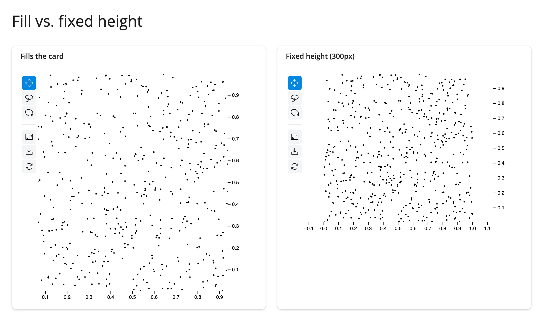
A plot fills its output (card or page) unless it has a height of its own. One quirk worth knowing: jupyter-scatter’s own default, Scatter(..., height=240), is specifically treated as “no height” and still fills – verified against current main: a plot built with height=240 fills a 372px card, while height=241 is honored as a fixed 241px plot. If you want a genuinely fixed 240px plot, ask for 241 (or anything else) instead. Once a plot has filled its output, Python can no longer resize it by setting .widget.height – the browser’s fit wins; choose the height at construction if you need a specific, unchanging size.
Gotchas and limitations
Verified on current main (shinywidgets, jupyter-scatter 1.0.1):
- At most 2 distinct data dimensions can drive color/size/opacity at once. A third distinct column raises
AssertionError: Only 2 data encodings are supportedat render time. Reuse a dimension across channels (as in the encodings example) to combine more than two visual channels. height=240is treated as “unspecified.” It’s jupyter-scatter’s own default, and shinywidgets can’t tell it apart from a user not setting a height at all, so a plot built withheight=240still fills its container. See Layout and sizing.selectionholds row positions, not index labels, unless theScatterwas built withdata_use_index=True. Passing index labels from a non-default-indexed frame into.widget.selectionselects the wrong rows silently (no error) and can make.zoom(to=...)raise out-of-range errors.- Selections over roughly 3 million points can exceed Shiny’s default 16 MiB websocket message limit, disconnecting the session (the selection array is base64-encoded JSON, not a binary frame). This is documented on the
render_jscatterclass itself; raise the limit withshiny run --ws-max-size <bytes>if your app lassoes selections at that scale. Not independently re-triggered at that scale in this pass – seeNOTES.md. jscatter.compose()and.link()return a plainipywidgets.GridBox, not aJupyterScatter, so@render_jscattercan’t render their result directly (it isn’t aScatter/JupyterScatter). Use@render_widgetinstead if you wantcompose()’s side-by-side layout (it won’t get fill behavior or theselected()accessor), or render the plots as separate@render_jscatteroutputs and link them in Python, as in Coordinating multiple views – which also composes more flexibly with the rest of a Shiny layout.- Fixed, compared to the earlier PR-review report: the jupyter-scatter toolbar’s own “Full Screen” button used to leave a filling plot’s canvas stuck at the wrong size after exiting fullscreen. Re-verified on current
main: entering and exiting fullscreen now leaves the canvas correctly tracking its container (tests/playwright/render_jscatter/test_render_jscatter.py::test_jscatter_fills_again_after_its_fullscreen_button, and reproduced independently for this guide).
Gallery candidates
Template: linked scatter plots with a selection table
gallery/template_linked_scatter.py – two linked jscatter plots (weight vs. MPG, horsepower vs. MPG) sharing a lasso selection, plus a table of the selected rows. A clean ~80-line starting point for any “explore two views of the same rows” app; swap in your own data frame and column names.
Showcase: 300,000 cells, lasso to explore
gallery/showcase_single_cell_atlas.py – a synthetic single-cell “atlas” explorer: two linked 300,000-point plots (a UMAP-like embedding and two marker genes), a live composition panel, a “color by” switch that restyles both plots in place, and a button that finds the top 1% of a marker gene from Python, selects those cells, and flies the camera to them.
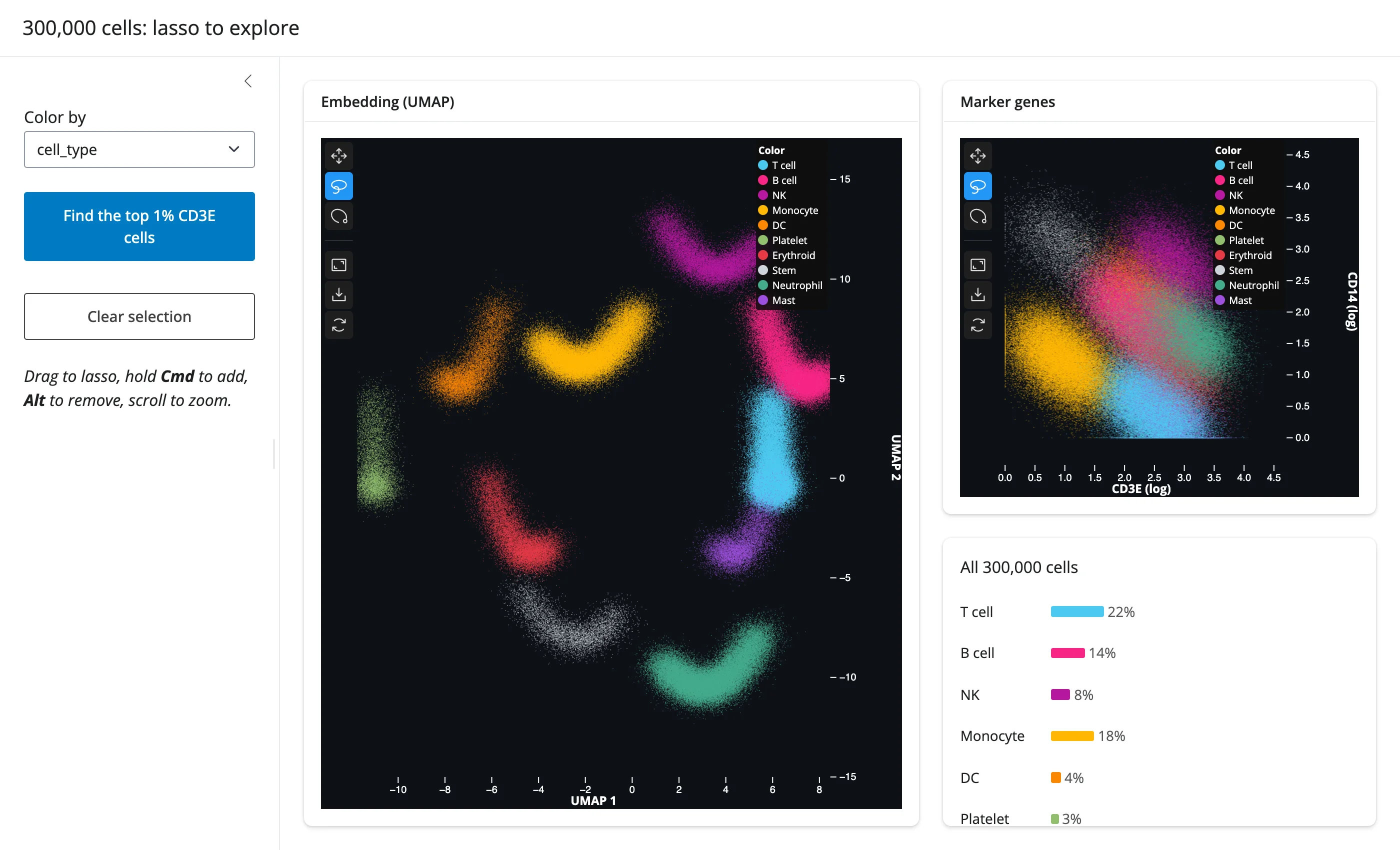
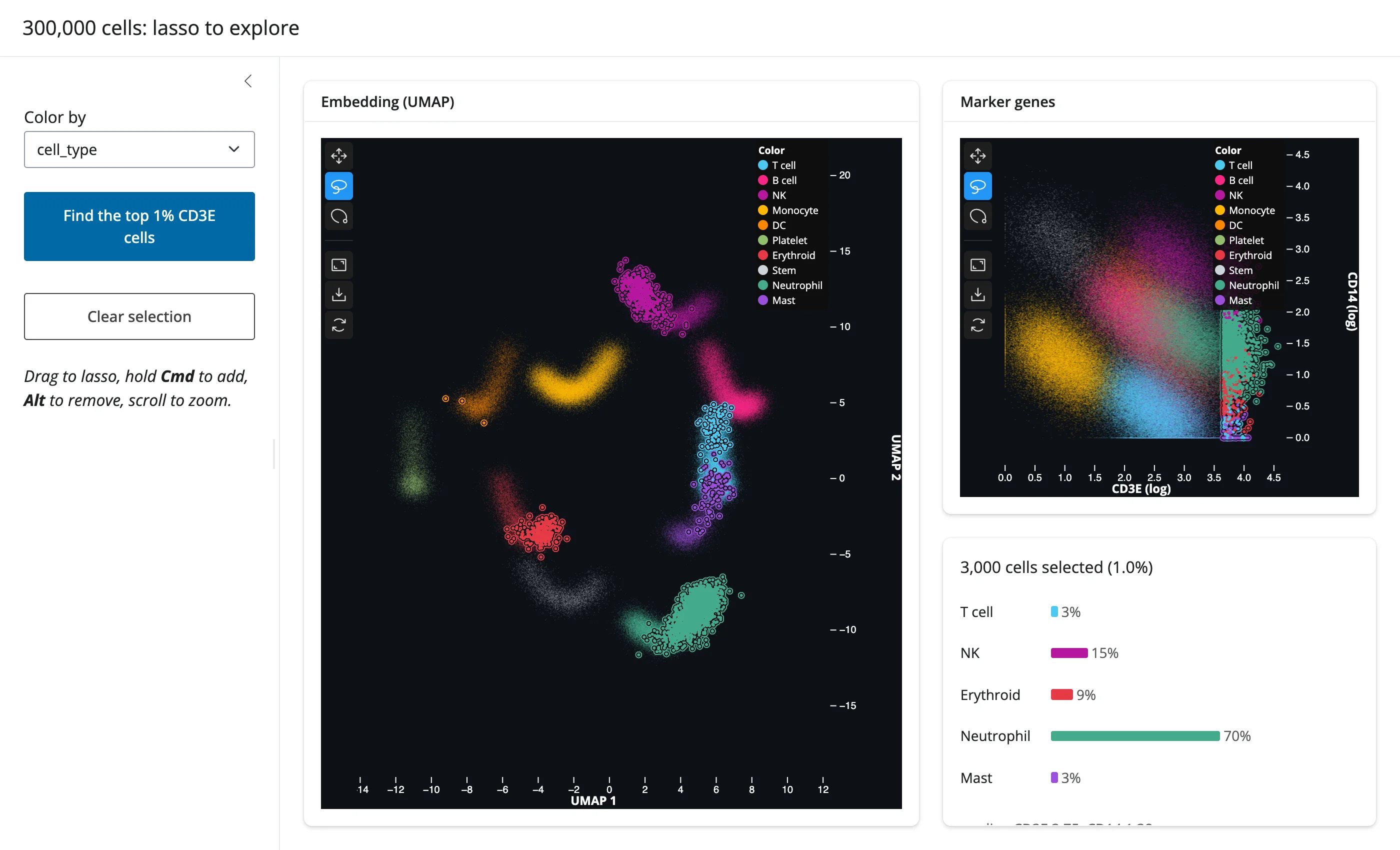
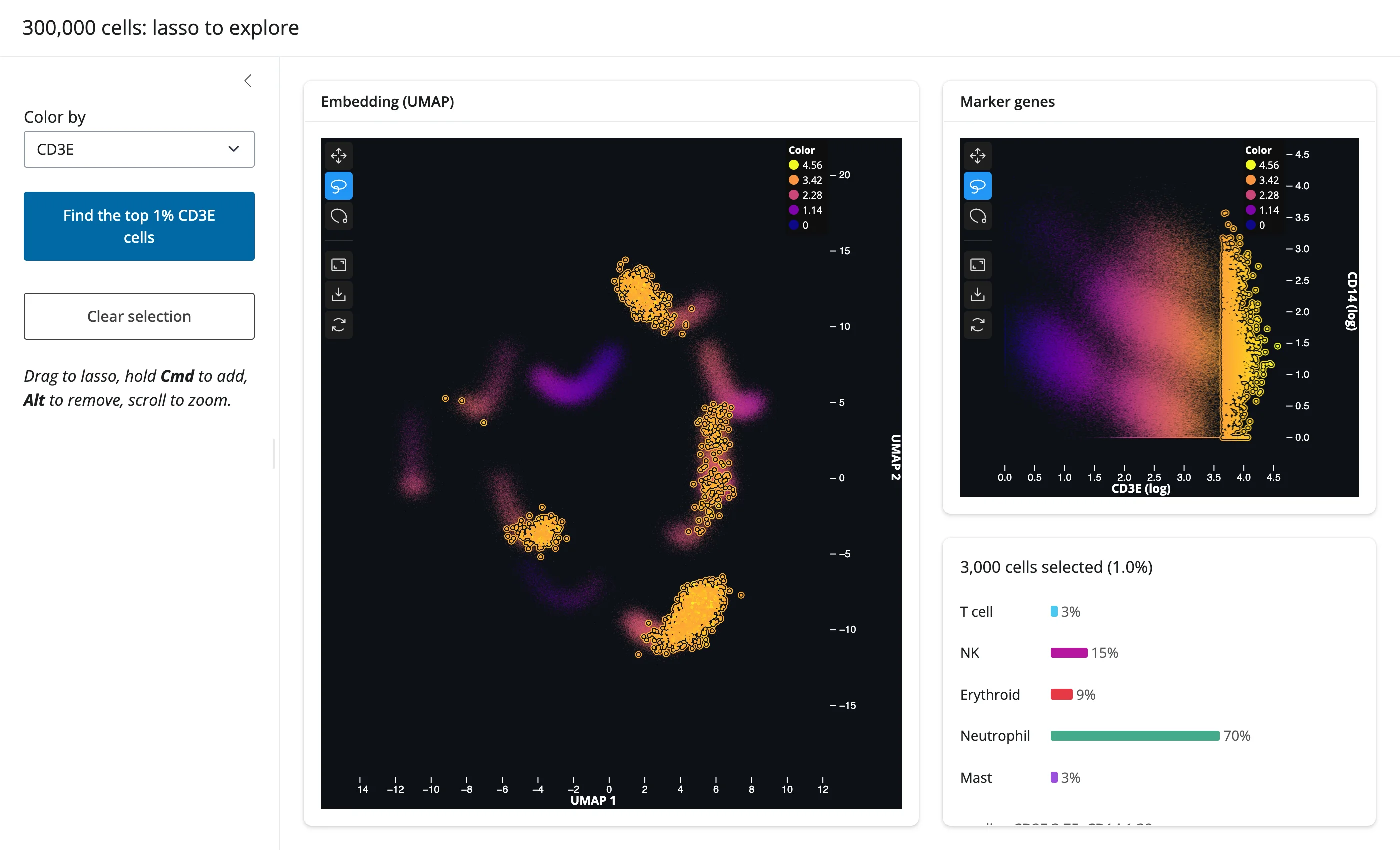
This exercises nearly everything in this guide at once: the selected() accessor, linked brushing across two plots, in-place restyling, and Python-driven selection plus an animated .zoom(). The “color by” dropdown restyles both plots without re-sending any of the 300,000 points’ coordinates (below, colored by the CD3E marker instead of cell type, selection preserved):
Learn more
- jupyter-scatter documentation – the full
ScatterAPI, including connections (connect_by), annotations, and label placement, none of which are covered above. - regl-scatterplot, the WebGL renderer jupyter-scatter is built on, for the mechanics of how it stays fast at scale.
- itables guide and ipydatagrid guide, for the table side of the linked-view patterns above.
- plotly guide and altair guide, for scatter plots with more chart types and moderate data sizes.
- embedding-atlas guide, for SQL-backed cross-filtering across many linked charts rather than a single scatter plot.