K3D

A GPU 3D scene in a Shiny output – millions of points, real terrain, volumes, and meshes, orbited by the user and driven from Python.

K3D Jupyter is a 3D plotting library built on WebGL and three.js, maintained by the K3D-tools project. It is the only widget in this roster built specifically for scientific 3D: point clouds, triangle meshes, volumetric data, isosurfaces, vector fields, and voxel grids all share one Plot scene, one camera, and one GPU renderer. Where plotly’s scatter_3d or pythreejs’s low-level scene graph cover part of this space, K3D is built around a small set of high-level drawable factories (k3d.points, k3d.surface, k3d.volume, k3d.marching_cubes, …) that render fast at real data sizes – a million-point cloud orbits smoothly in the browser.

@render_k3d accepts a k3d.Plot (what k3d.plot() returns) or a bare drawable such as k3d.points(...), which it places on a new plot for you (mirroring what K3D’s own Jupyter display does). It fills its container by default; pass height= to k3d.plot() for a fixed pixel size instead. The one accessor, camera(), turns the user’s orbit/pan/zoom into a value you can read like an input – feed it to another view, a caption, or a “what’s visible” computation. K3D has no click/select accessor (see “Beyond the accessors” below) – you wire picking yourself with K3D’s own click_callback, which this guide also covers because it is how most interactive K3D apps actually work.

Choose K3D when the point is a real 3D scene – spatial data, simulation output, a surface or a volume – that users should be able to fly through and inspect. For a quick 3D scatter next to 2D charts, plotly’s scatter_3d is lighter weight. For geographic point clouds and vector layers, see lonboard; for medical imaging volumes specifically, see niivue. For a lower-level three.js scene graph (custom geometries, non-K3D materials), see pythreejs.

hero

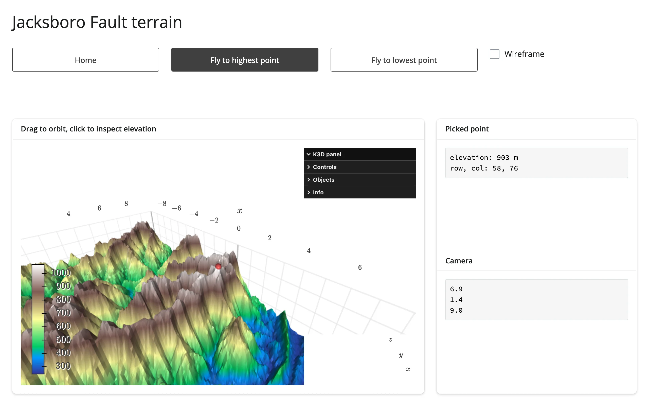
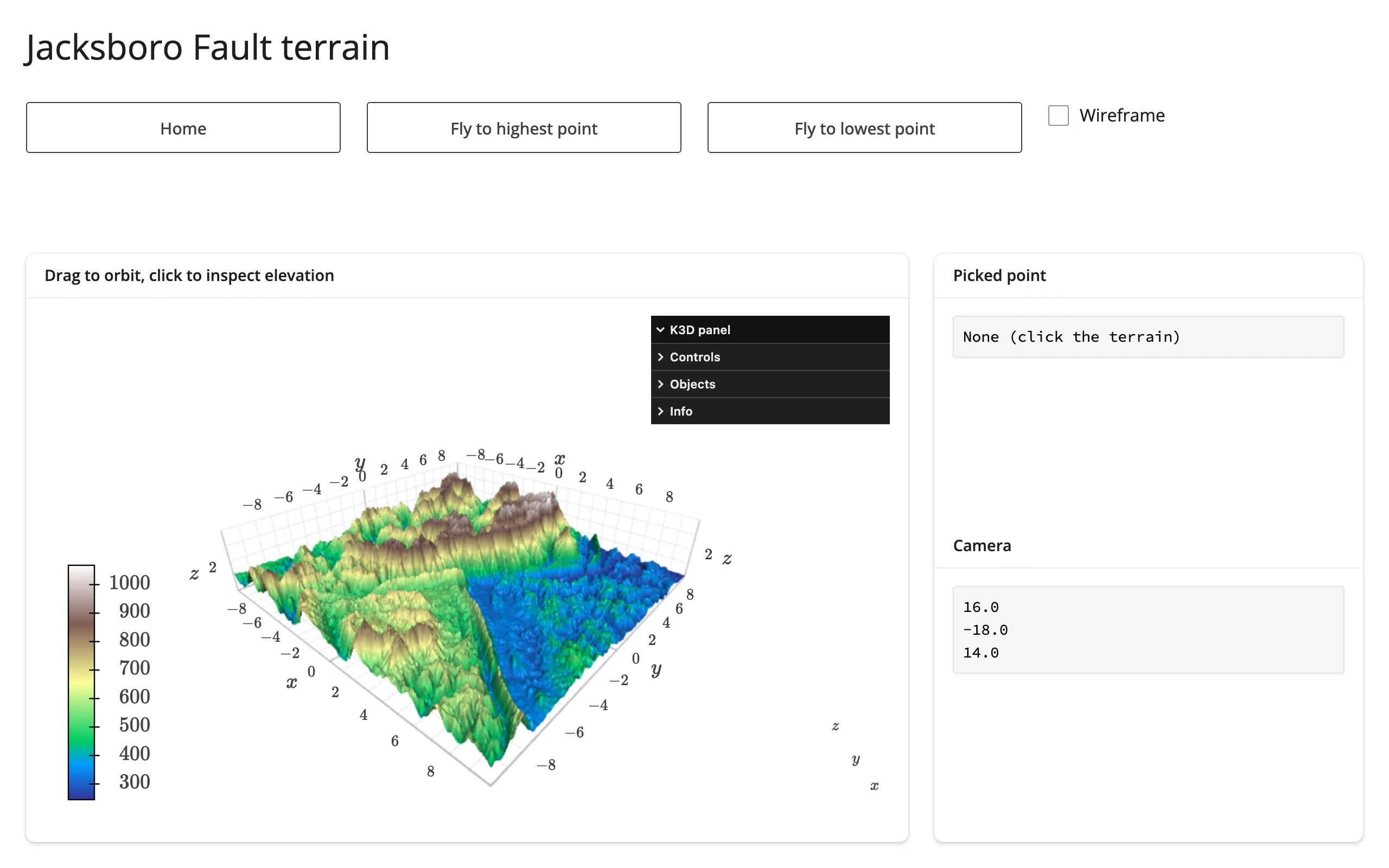
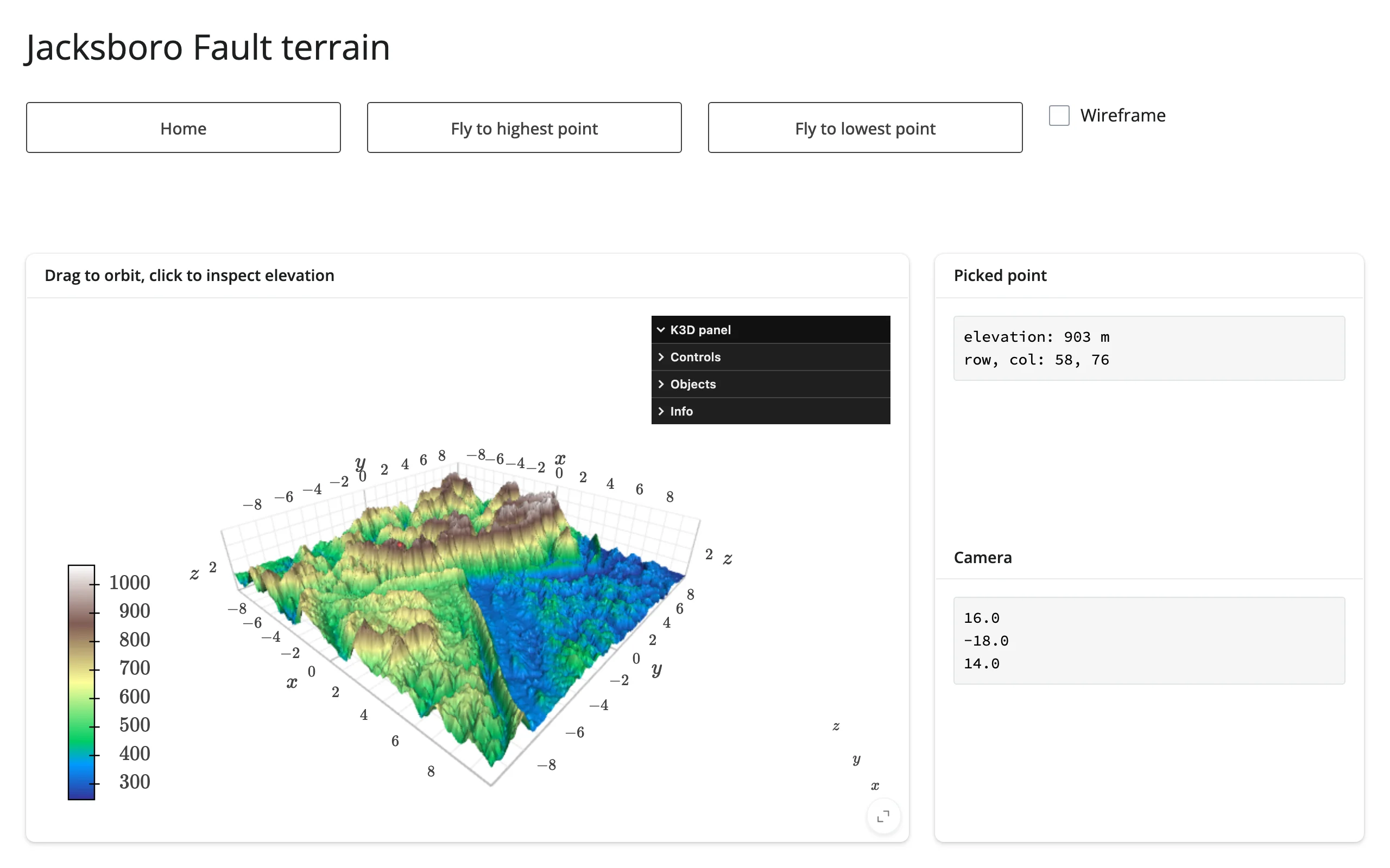
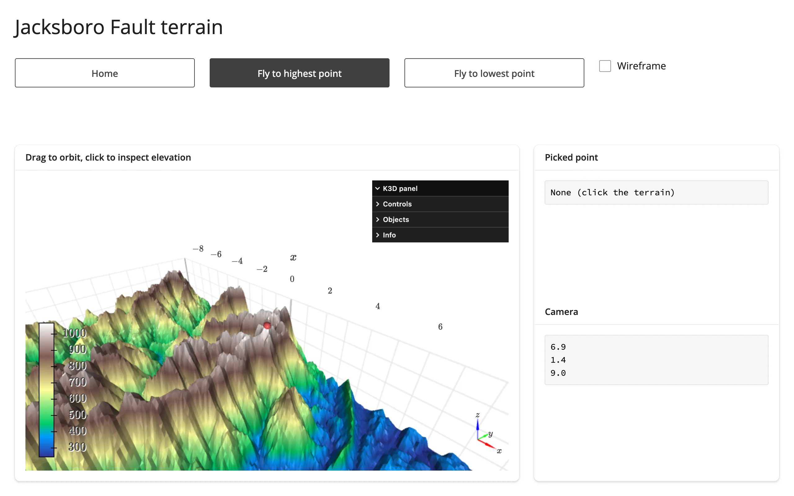
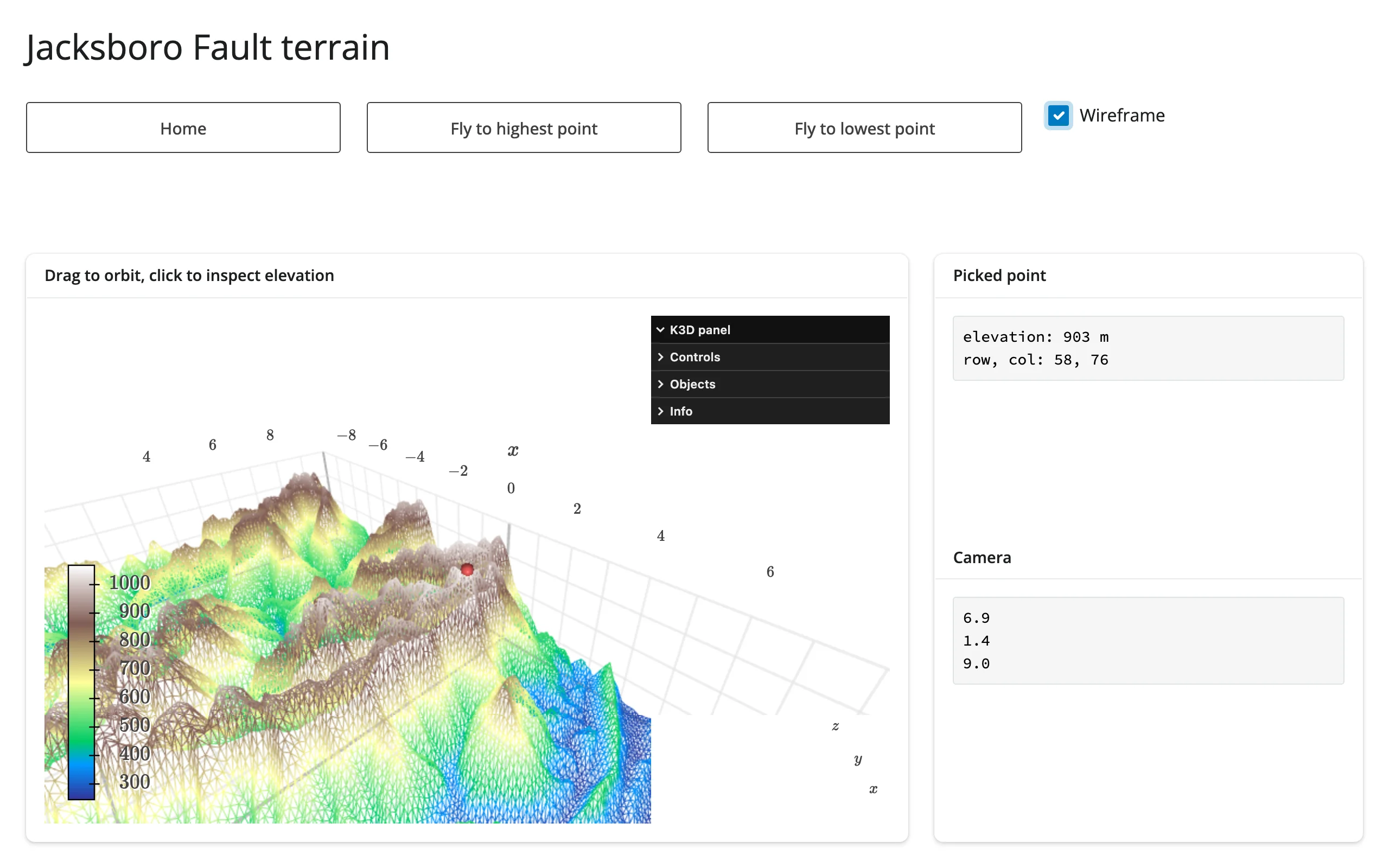
A real DEM (Jacksboro Fault, Texas), clicked to read elevation, flown to its highest point – in place, no re-render. From gallery/showcase_terrain_explorer.py.

Installation

pip install 'shinywidgets[k3d]'

This installs k3d (tested against 3.2.0, the anywidget-based release). shinywidgets imports k3d.plot.Plot and k3d.factory.plot, paths specific to K3D 3.x – the older, ipywidgets-comm-based 2.x releases are not what this guide (or the renderer) targets.

Quick start

examples/01_quickstart.py22 lines

# Needs scikit-learn for the iris dataset:
#   uv run --with scikit-learn shiny run docs/widget-guides/k3d/examples/01_quickstart.py
from __future__ import annotations

import k3d
import numpy as np
from shiny.express import ui
from sklearn.datasets import load_iris
from shinywidgets import render_k3d

iris = load_iris(as_frame=True).frame
xyz = iris[["sepal length (cm)", "sepal width (cm)", "petal length (cm)"]].to_numpy(np.float32)
species_color = np.choose(iris["target"].to_numpy(), [0xE41A1C, 0x377EB8, 0x4DAF4A]).astype(np.uint32)

ui.page_opts(title="Iris in 3D", fillable=True)


@render_k3d
def plot():
    scene = k3d.plot()
    scene += k3d.points(xyz, colors=species_color, point_size=0.2, shader="3d")
    return scene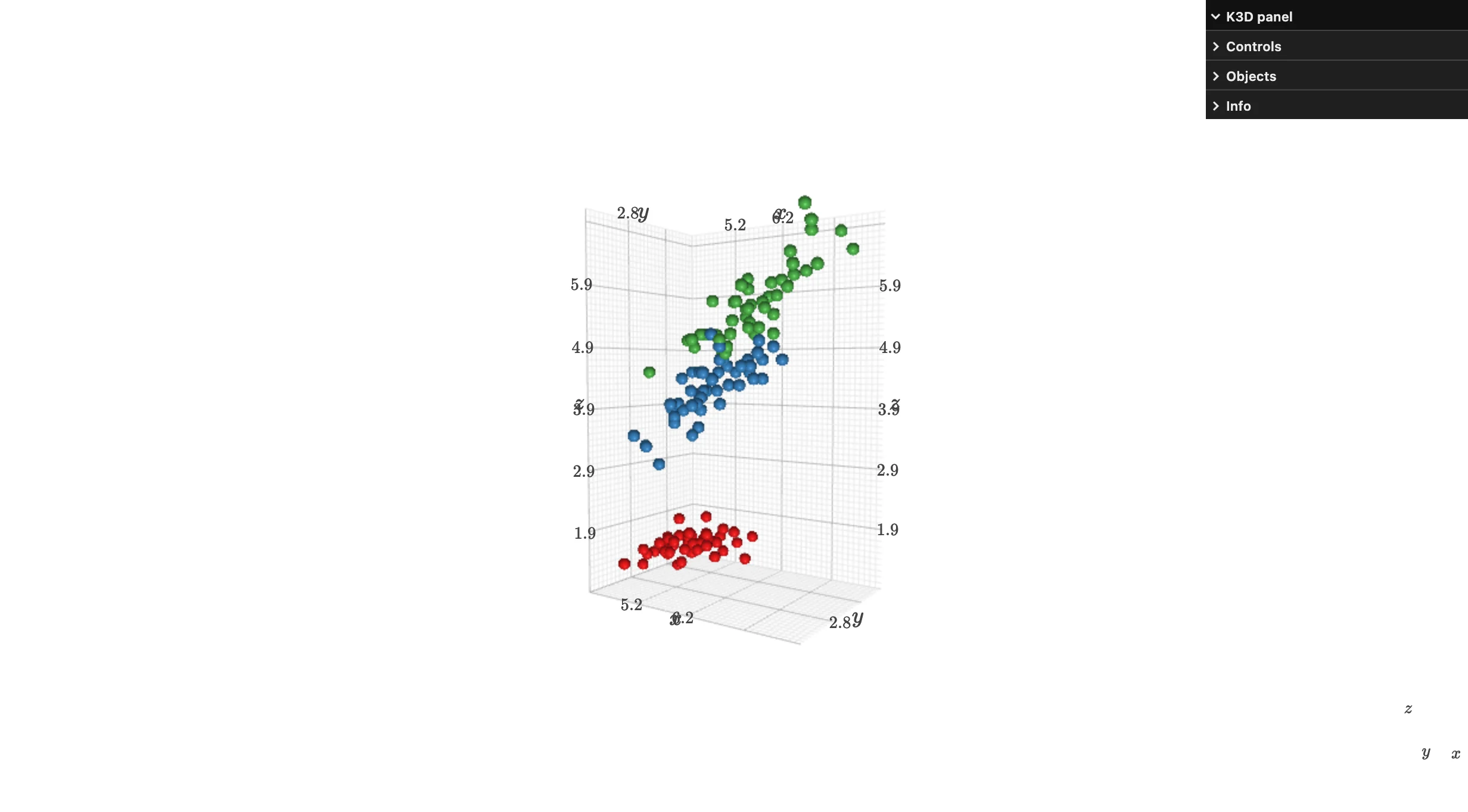

quickstart

k3d.plot() makes an empty scene; += adds drawables to it (it builds a Group under the hood, so fig1 += fig2 also works to combine two drawables). The plot fills its output with no extra sizing code, and the orbit/zoom/pan you see is free – K3D’s own trackball camera, not something shinywidgets adds.

What you can build

K3D’s drawable factories (k3d.points, k3d.surface, k3d.volume, k3d.marching_cubes, k3d.line, k3d.vectors, k3d.text) cover most of what a 3D scientific scene needs. Combine several in one Plot freely – each is independently addressable afterward via plot.objects[i].

A million points, still orbitable. shader="flat" (billboard sprites, no per-point lighting) is the fast path at this scale; attribute=/color_map= map a value to color, same idea as a c=/cmap= scatter:

examples/02_point_cloud_scale.py30 lines

from __future__ import annotations

import k3d
import numpy as np
from shiny.express import ui
from shinywidgets import render_k3d

N = 1_000_000
rng = np.random.default_rng(0)
xyz = (rng.normal(size=(N, 3)) * 3).astype(np.float32)
dist = np.linalg.norm(xyz, axis=1)

ui.page_opts(title=f"{N:,} points", fillable=True)


@render_k3d
def cloud():
    # An explicit camera (rather than auto-fit's zoomed-out default) composes
    # a tighter, more legible shot of the cluster.
    scene = k3d.plot(camera_auto_fit=False)
    scene.camera = [24, 19, 14, 0, 0, 0, 0, 0, 1]
    scene += k3d.points(
        xyz,
        point_size=0.03,
        shader="flat",
        attribute=dist,
        color_map=k3d.matplotlib_color_maps.Viridis,
        opacity=0.6,
    )
    return scene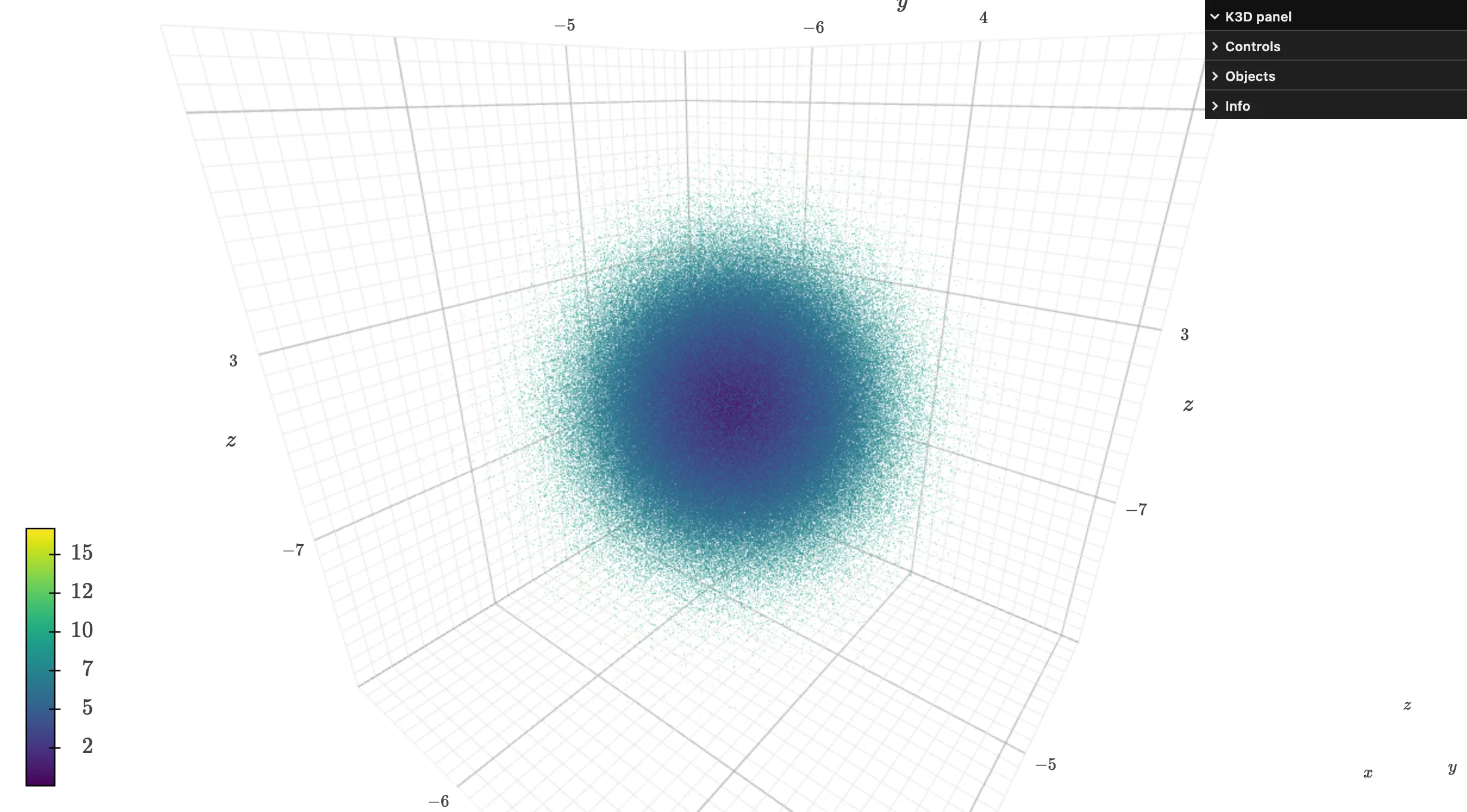

a million points

A million points render and stay orbitable at interactive frame rates (verified on current main; SwiftShader software rendering, no GPU – see Gotchas). camera_auto_fit’s default framing leaves generous margin around the data (camera_reset(factor=1.5)’s default); setting plot.camera explicitly, as above, composes a tighter shot.

A real terrain surface, colored by elevation. k3d.surface turns a 2D height array into a 3D surface; bounds=[xmin, xmax, ymin, ymax] sets its footprint (the default is a unit square centered on the origin):

examples/03_terrain_surface.py44 lines

# Uses a real DEM (elevation grid) that ships inside matplotlib's sample data.
from __future__ import annotations

import k3d
import matplotlib.cbook as cbook
import numpy as np
from shiny.express import ui
from shinywidgets import render_k3d

elevation = cbook.get_sample_data("jacksboro_fault_dem.npz")["elevation"][::2, ::2].astype(np.float32)
relief = (elevation - elevation.min()) / (elevation.max() - elevation.min()) * 4.0

peak_row, peak_col = np.unravel_index(np.argmax(elevation), elevation.shape)
nrows, ncols = elevation.shape
peak_xyz = (
    -10 + peak_col / (ncols - 1) * 20,
    -10 + peak_row / (nrows - 1) * 20,
    float(relief[peak_row, peak_col]) + 0.3,
)

ui.page_opts(title="Jacksboro Fault DEM", fillable=True)


@render_k3d
def terrain():
    scene = k3d.plot(camera_auto_fit=False)
    scene.camera = [16, -18, 14, 0, 0, 1, 0, 0, 1]
    scene += k3d.surface(
        relief,
        bounds=[-10, 10, -10, 10],
        attribute=elevation,
        color_map=k3d.matplotlib_color_maps.Terrain,
        color_range=[float(elevation.min()), float(elevation.max())],
    )
    # is_html=True avoids k3d.text's default LaTeX rendering, which drops spaces
    # (e.g. "Highest point" renders as "Highestpoint")
    scene += k3d.text(
        "Highest point (1068 m)",
        position=peak_xyz,
        color=0x000000,
        label_box=True,
        is_html=True,
    )
    return scene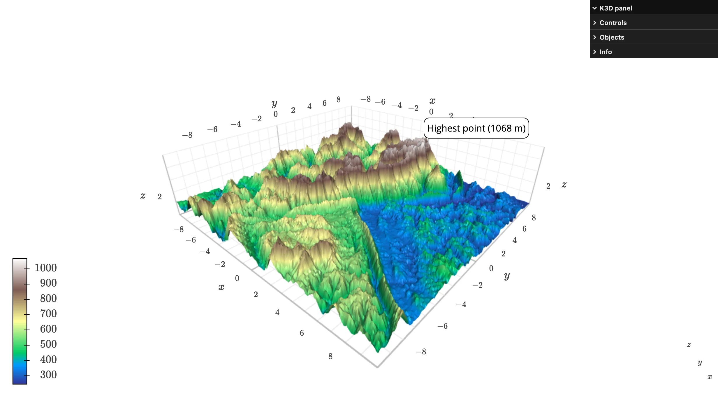

terrain surface

relief (the surface’s z-height) is scaled for a pleasant vertical exaggeration; attribute=elevation keeps the color mapped to the true elevation in meters, independent of that scaling – a common pattern when the natural x/y/z units would otherwise make the terrain look nearly flat.

An isosurface from a scalar field. k3d.marching_cubes extracts the surface where a 3D scalar field crosses level – here, the implicit equation of a torus:

examples/04_mesh_isosurface.py23 lines

from __future__ import annotations

import k3d
import numpy as np
from shiny.express import ui
from shinywidgets import render_k3d

n = 80
lin = np.linspace(-2, 2, n, dtype=np.float32)
x, y, z = np.meshgrid(lin, lin, lin, indexing="ij")
major_radius, minor_radius = 1.0, 0.4
field = (np.sqrt(x**2 + y**2) - major_radius) ** 2 + z**2 - minor_radius**2

ui.page_opts(title="An isosurface, from a scalar field", fillable=True)


@render_k3d
def torus():
    scene = k3d.plot()
    scene += k3d.marching_cubes(
        field, level=0.0, color=0x2E86AB, flat_shading=False
    )
    return scene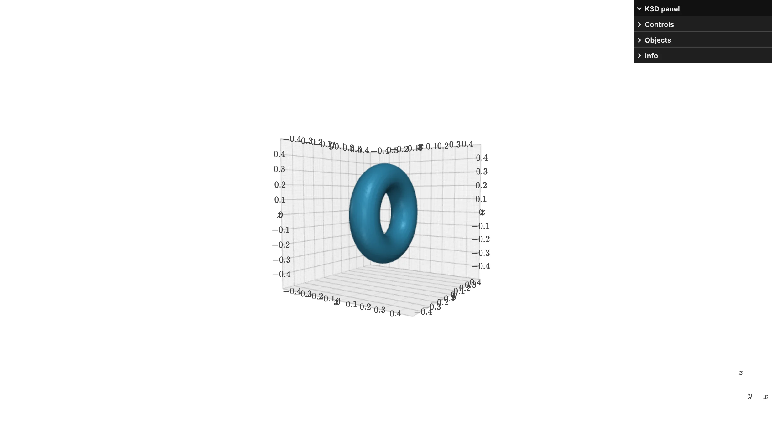

isosurface mesh

marching_cubes ignores the field’s own coordinate range – the mesh always comes out in a unit cube centered on the origin (use spacings_x/_y/_z or a model_matrix to rescale it). A plain triangle mesh you already have (e.g. loaded from an STL) works the same way through k3d.mesh(vertices, indices).

Volumetric rendering. k3d.volume ray-marches a 3D scalar field directly – no surface extraction, so it shows density gradients an isosurface would hide:

examples/05_volume.py28 lines

from __future__ import annotations

import k3d
import numpy as np
from shiny.express import ui
from shinywidgets import render_k3d

n = 64
lin = np.linspace(-1, 1, n, dtype=np.float32)
x, y, z = np.meshgrid(lin, lin, lin, indexing="ij")
blobs = [(-0.3, -0.2, 0.1, 0.25), (0.3, 0.2, -0.1, 0.3), (0.0, 0.4, 0.3, 0.2)]
density = np.zeros((n, n, n), dtype=np.float32)
for cx, cy, cz, spread in blobs:
    density += np.exp(-((x - cx) ** 2 + (y - cy) ** 2 + (z - cz) ** 2) / (2 * spread**2))

ui.page_opts(title="Volumetric density field", fillable=True)


@render_k3d
def nebula():
    scene = k3d.plot()
    scene += k3d.volume(
        density,
        color_map=k3d.matplotlib_color_maps.Plasma,
        color_range=[0.1, density.max()],
        alpha_coef=25,
    )
    return scene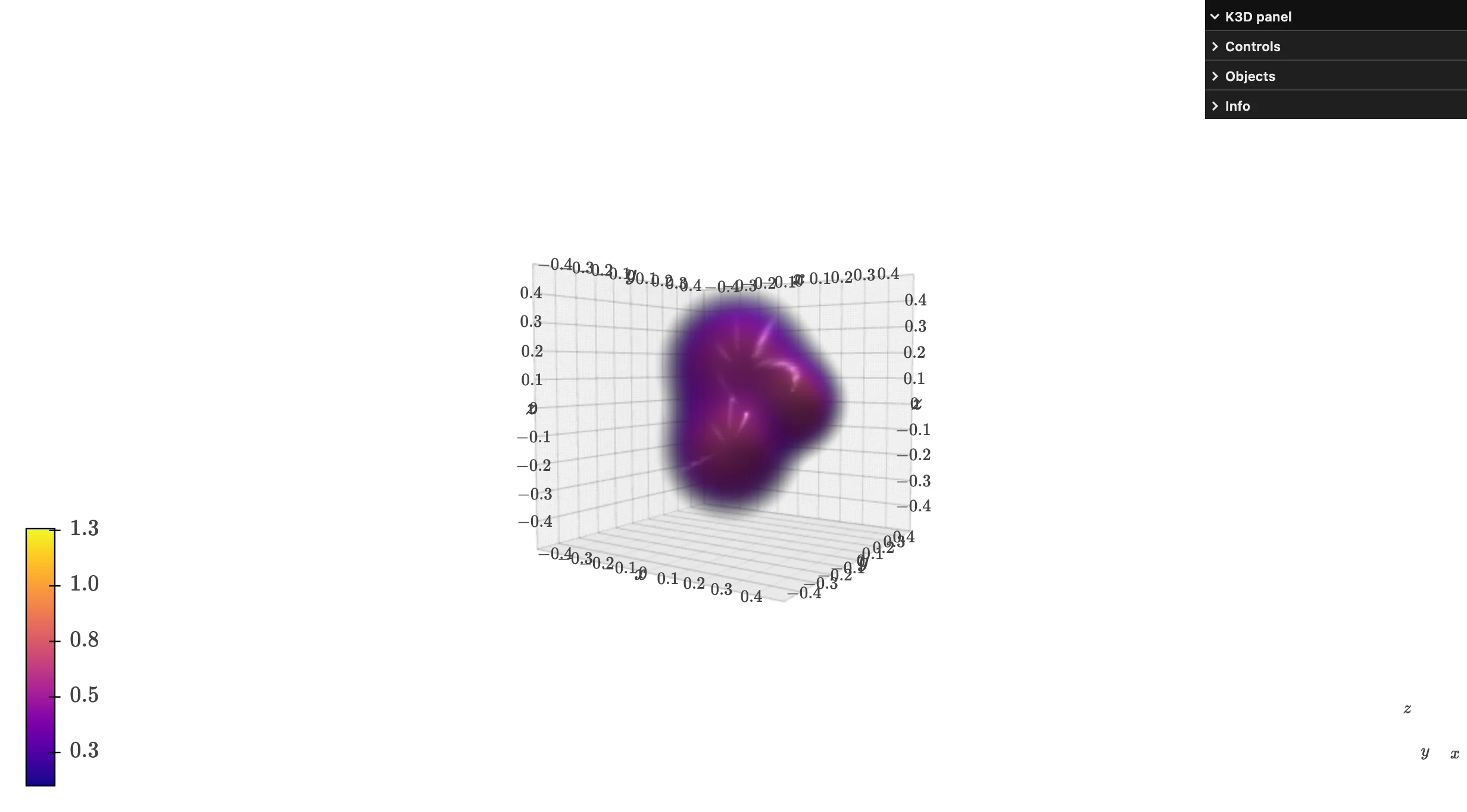

volume

alpha_coef controls overall opacity (higher = more opaque, so thin wisps vanish before dense cores do); raise samples (default 512) for a less noisy render at a frame-rate cost.

Lines and vector fields. k3d.line draws a polyline; k3d.vectors draws arrows from origins along vectors – here, a classic chaotic trajectory with local velocity vectors sampled along it:

examples/06_lines_vectors.py33 lines

from __future__ import annotations

import k3d
import numpy as np
from shiny.express import ui
from shinywidgets import render_k3d


def lorenz_step(xyz: np.ndarray, s: float = 10, r: float = 28, b: float = 8 / 3) -> np.ndarray:
    x, y, z = xyz
    return np.array([s * (y - x), x * (r - z) - y, x * y - b * z])


dt, n = 0.01, 4000
path = np.empty((n, 3), dtype=np.float32)
path[0] = [0.1, 0.0, 0.0]
for i in range(1, n):
    path[i] = path[i - 1] + lorenz_step(path[i - 1]) * dt

# Local velocity (the Lorenz system's own derivative) at a few points, scaled
# down for display -- vectors show direction/speed along the trajectory.
sample = path[::400]
velocity = np.array([lorenz_step(p) for p in sample], dtype=np.float32) * 0.12

ui.page_opts(title="Lorenz attractor", fillable=True)


@render_k3d
def attractor():
    scene = k3d.plot()
    scene += k3d.line(path, color=0x1F77B4, shader="thick", width=0.3)
    scene += k3d.vectors(sample, velocity, color=0xE45756, head_size=4.0, line_width=0.6)
    return scene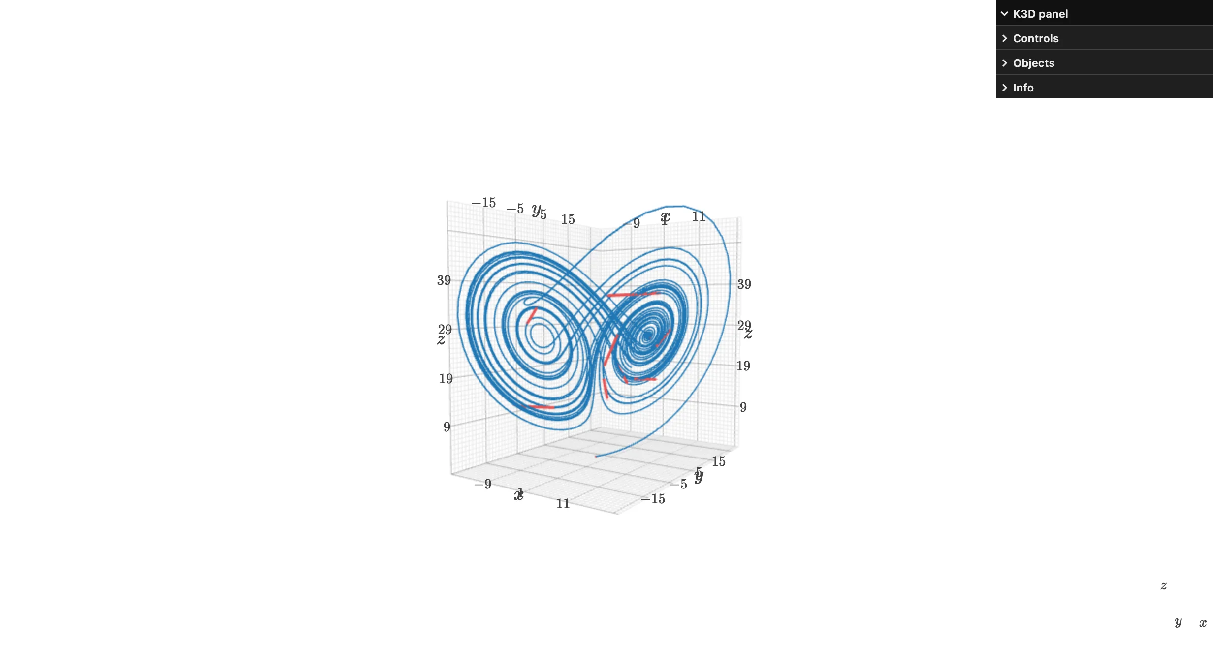

lines and vectors

Time-keyed animation. Any synced trait accepts a {time: value} dict instead of a plain value; K3D interpolates between keyframes as plot.time advances. start_auto_play()/stop_auto_play() drive time automatically at plot.fps (default 25/s):

examples/07_animation.py54 lines

from __future__ import annotations

import k3d
import numpy as np
from shiny import reactive
from shiny.express import input, render, ui
from shinywidgets import render_k3d

N_STEPS = 60
t = np.linspace(0, 2 * np.pi, N_STEPS, endpoint=False)


def orbit(radius: float, speed: float) -> dict[float, np.ndarray]:
    xs, ys = radius * np.cos(speed * t), radius * np.sin(speed * t)
    pos = np.stack([xs, ys, np.zeros_like(xs)], axis=1).astype(np.float32)
    return {float(i) / N_STEPS: pos[i : i + 1] for i in range(N_STEPS)}


ui.page_opts(title="Orbits, driven by a time-keyed trait", fillable=True)
ui.input_action_button("play", "Play")
ui.input_action_button("pause", "Pause")


@render_k3d
def orbits():
    scene = k3d.plot(camera_auto_fit=False, grid_visible=False)
    scene.camera = [0, 0, 14, 0, 0, 0, 0, 1, 0]
    scene += k3d.points([[0, 0, 0]], point_size=0.8, color=0xFFC300, shader="3d")
    scene += k3d.points(orbit(3, 1), point_size=0.4, color=0x1F77B4, shader="3d")
    scene += k3d.points(orbit(5, 0.5), point_size=0.5, color=0xE45756, shader="3d")
    return scene


# start_auto_play()/stop_auto_play() now reach the browser even when called
# directly in the render function (the comm-not-open-yet case no longer drops
# the message) -- but a call made before the k3d view has connected in the
# browser is dropped silently by k3d's JS, and the render function is always
# that early. Calls from later effects work; buttons are the robust version
# of "later", so wire them to buttons.
@reactive.effect
@reactive.event(input.play)
def _play():
    orbits.widget.start_auto_play()


@reactive.effect
@reactive.event(input.pause)
def _pause():
    orbits.widget.stop_auto_play()


@render.text
def time():
    return f"plot.time = {orbits.read('time'):.2f}"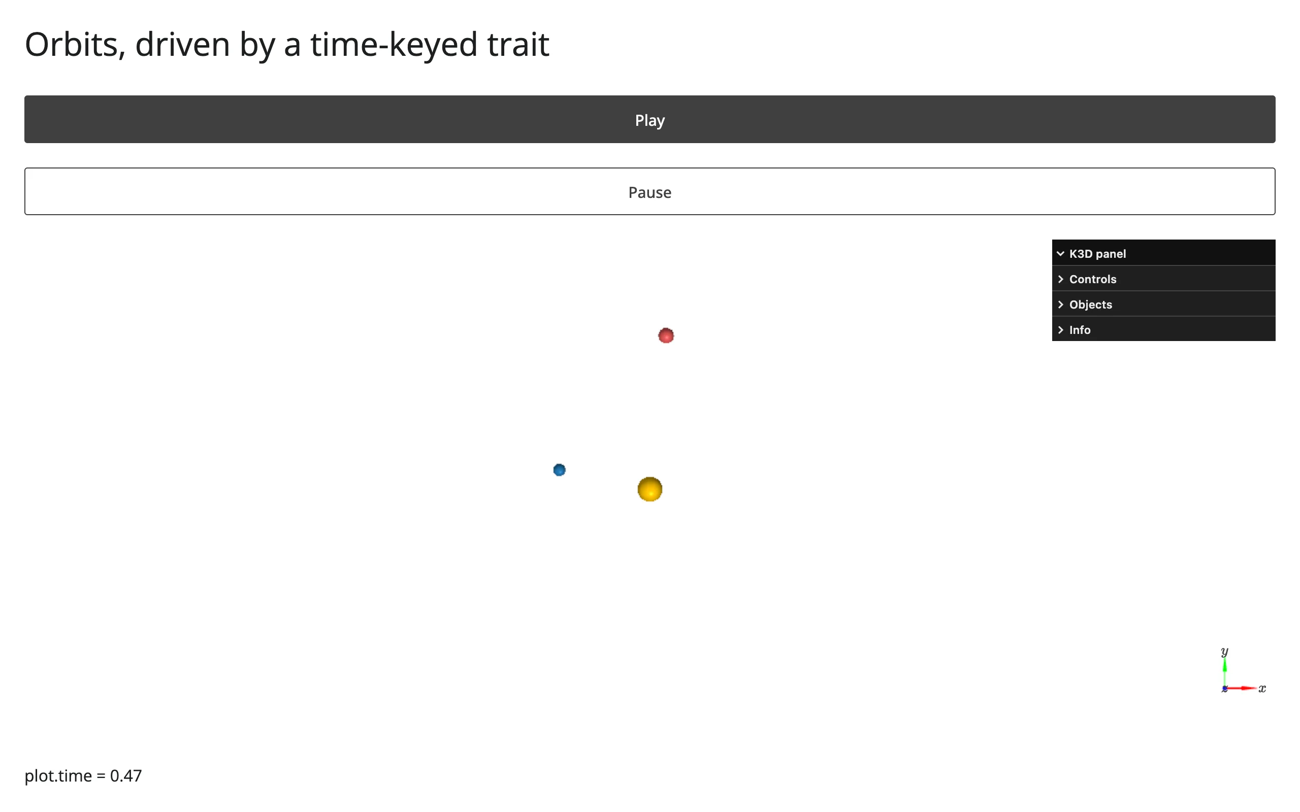

animation playing

The comment above matters in practice: calling scene.start_auto_play() directly inside the render function (before returning) used to send nothing at all, because the comm was still a placeholder at that point – that’s fixed. Verified on current main: the message is now delivered to the browser even from the render function (confirmed with a websocket capture), but k3d’s JS registers its custom-message handler per view when the view connects, so a message that arrives before then is dropped silently and playback never starts. The render function (and a bare startup effect) is always that early. Once the view is up, any call works – no user gesture needed; an effect delayed a few seconds with reactive.invalidate_later() starts playback fine. Buttons are simply the most robust form of “later”. See Gotchas.

Reacting to user interaction

Accessor reference

Accessor	Returns	Before any interaction	Across re-render	Default rate policy
camera()	list[float] of 9 (eye, target, up)	cancels until the browser’s auto-fit reports	re-seeded from the new plot	none (K3D already throttles to ~200ms upstream)

Call it from any reactive context (a @render.* function, @reactive.calc, or @reactive.effect); it invalidates that context whenever the camera changes, the same way input.x() does. It can also be read by name – scene.read("camera") – which is equivalent but useful when reading accessors generically (e.g., logging every accessor on an output).

camera()

examples/08_camera_accessor.py28 lines

from __future__ import annotations

import k3d
import numpy as np
from shiny.express import render, ui
from shinywidgets import render_k3d

rng = np.random.default_rng(0)
xyz = (rng.normal(size=(4000, 3))).astype(np.float32)

ui.page_opts(title="camera() follows every orbit", fillable=True)

with ui.layout_columns(col_widths=[8, 4]):
    with ui.card(full_screen=True):
        ui.card_header("Drag to orbit, scroll to zoom")

        @render_k3d
        def scene():
            plot = k3d.plot()
            plot += k3d.points(xyz, point_size=0.08, color=0x4C78A8, shader="3d")
            return plot

    with ui.card():
        ui.card_header("scene.camera()")

        @render.code
        def camera_out():
            return "\n".join(f"{v:.2f}" for v in scene.camera())

Before orbiting, and after a drag:

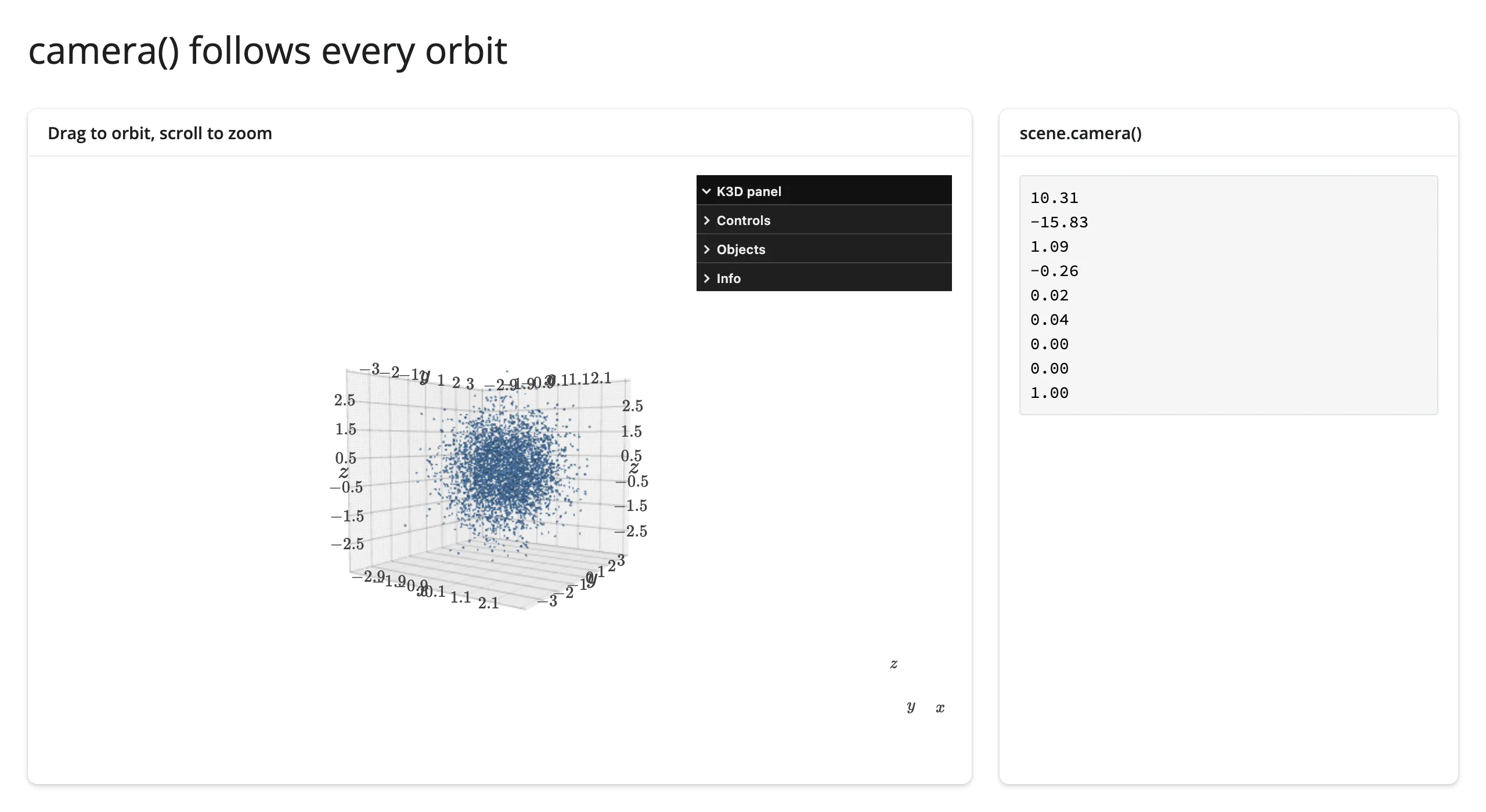
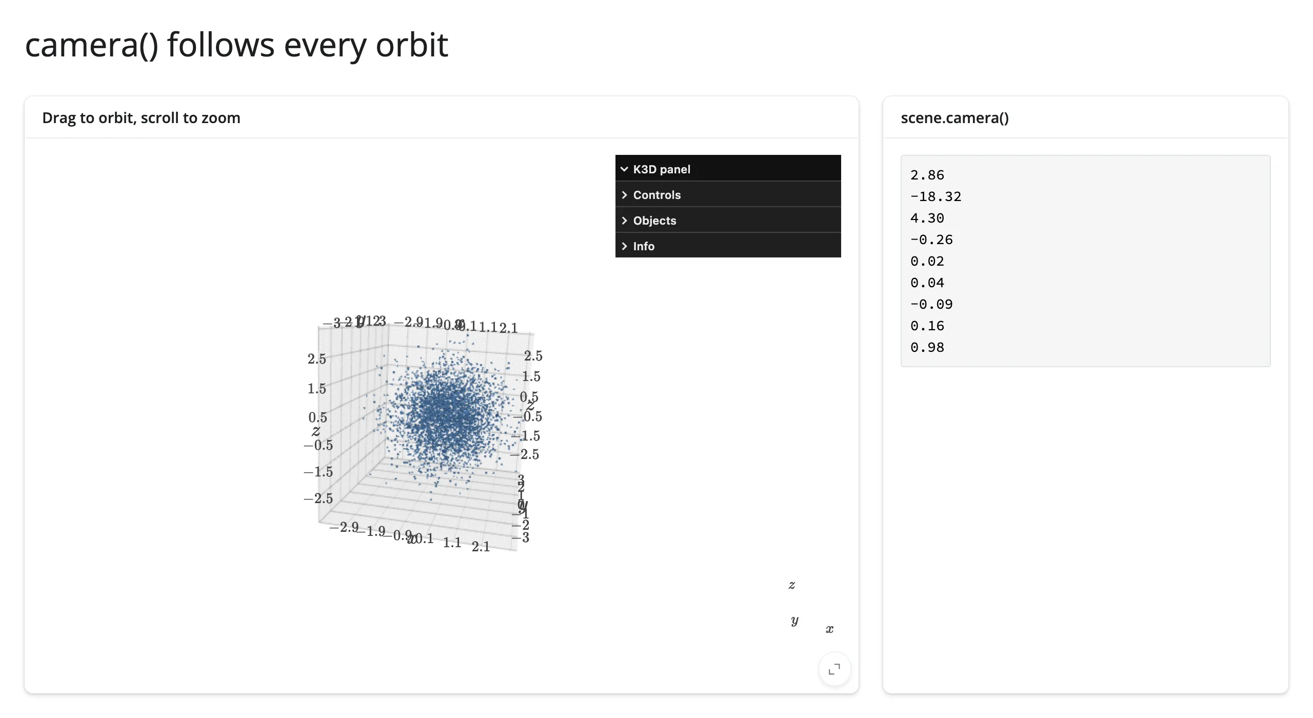
Verified on current main: camera() never returns None. Before the browser’s auto-fit reports (which, with the default camera_auto_fit=True, happens within the same render pass the user sees), reading it cancels the calling context, the same way req(False) does; downstream outputs just wait, with no error. With camera_auto_fit=False and no explicit plot.camera assigned, it cancels forever – seed plot.camera yourself (as every example above does once auto-fit isn’t wanted). Reading the raw trait instead (plot.read("camera"), or reactive_read(plot.widget, "camera")) shows the same thing as the sentinel: an empty list, [], until fitted.

Across a re-render, camera() re-seeds from the new plot rather than keeping the old orbit (verified: orbiting, then re-rendering with wider data, reports the new plot’s auto-fit framing, not the previous camera). It’s inherent widget state – like a map’s zoom or bounds – not a one-off interaction to preserve across a scene that no longer exists. If you want the old camera to carry over to a rebuilt scene, read it before the re-render and assign it back explicitly (new_plot.camera = old_camera), as examples/12_fly_to.py’s “Home” button and examples/13_sync_cameras.py both do.

Beyond the accessors: picking, and .read()

There is deliberately no clicked(). K3D only reports clicks through plot.mode = "callback" plus a click_callback on the clickable object – a user-visible change to the plot’s interaction mode (cursor behavior changes for everyone), which this design’s accessor model won’t make on your behalf. Wire it yourself:

examples/09_picking_callback.py53 lines

# k3d has no clicked() accessor (picking needs mode="callback", a user-visible
# change to the plot's interaction mode) -- wire k3d's own click_callback to a
# reactive.value instead.
from __future__ import annotations

import k3d
import numpy as np
from shiny import reactive
from shiny.express import render, ui
from shinywidgets import render_k3d

rng = np.random.default_rng(0)
xyz = (rng.normal(size=(300, 3)) * 2).astype(np.float32)

clicked = reactive.value(None)

ui.page_opts(title="Click a point", fillable=True)

with ui.layout_columns(col_widths=[8, 4]):
    with ui.card(full_screen=True):
        ui.card_header("plot.mode = 'callback': click a point")

        @render_k3d
        def scene():
            plot = k3d.plot(mode="callback")
            plot += k3d.points(
                xyz,
                point_size=0.15,
                color=0x4C78A8,
                click_callback=lambda info: clicked.set(info),
            )
            plot += k3d.points(xyz[:1], point_size=0.3, color=0xE45756, visible=False)
            return plot

        @reactive.effect
        def _highlight():
            info = clicked()
            if info is None:
                return
            highlight = scene.widget.objects[1]
            highlight.positions = np.array([info["position"]], dtype=np.float32)
            highlight.visible = True

    with ui.card():
        ui.card_header("k3d's own click_callback, not an accessor")

        @render.code
        def out():
            info = clicked()
            if info is None:
                return "None (click a point)"
            position = [round(v, 2) for v in info["position"]]
            return f"index: {info['index']}\nposition: {position}"

Before and after clicking a point:

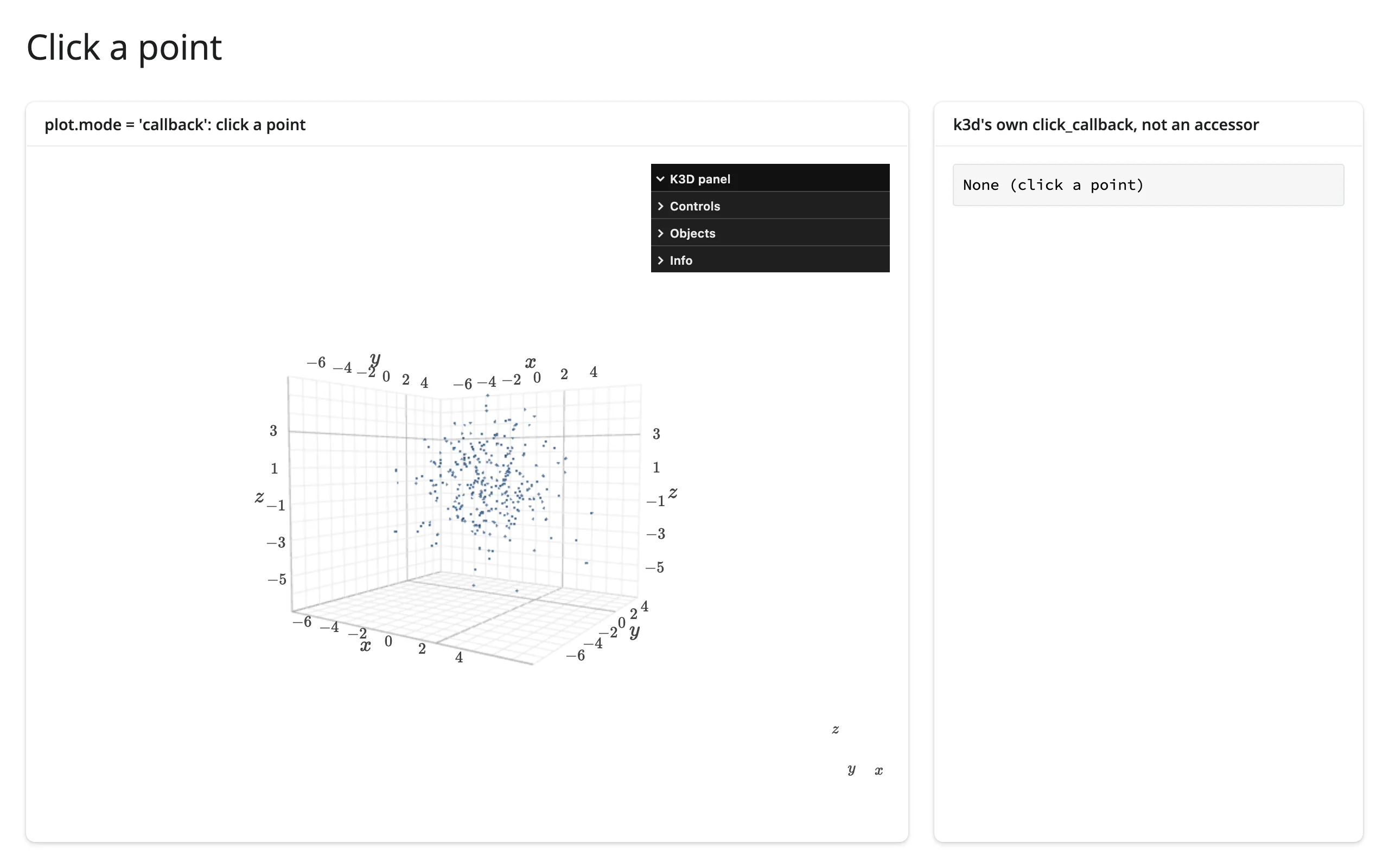
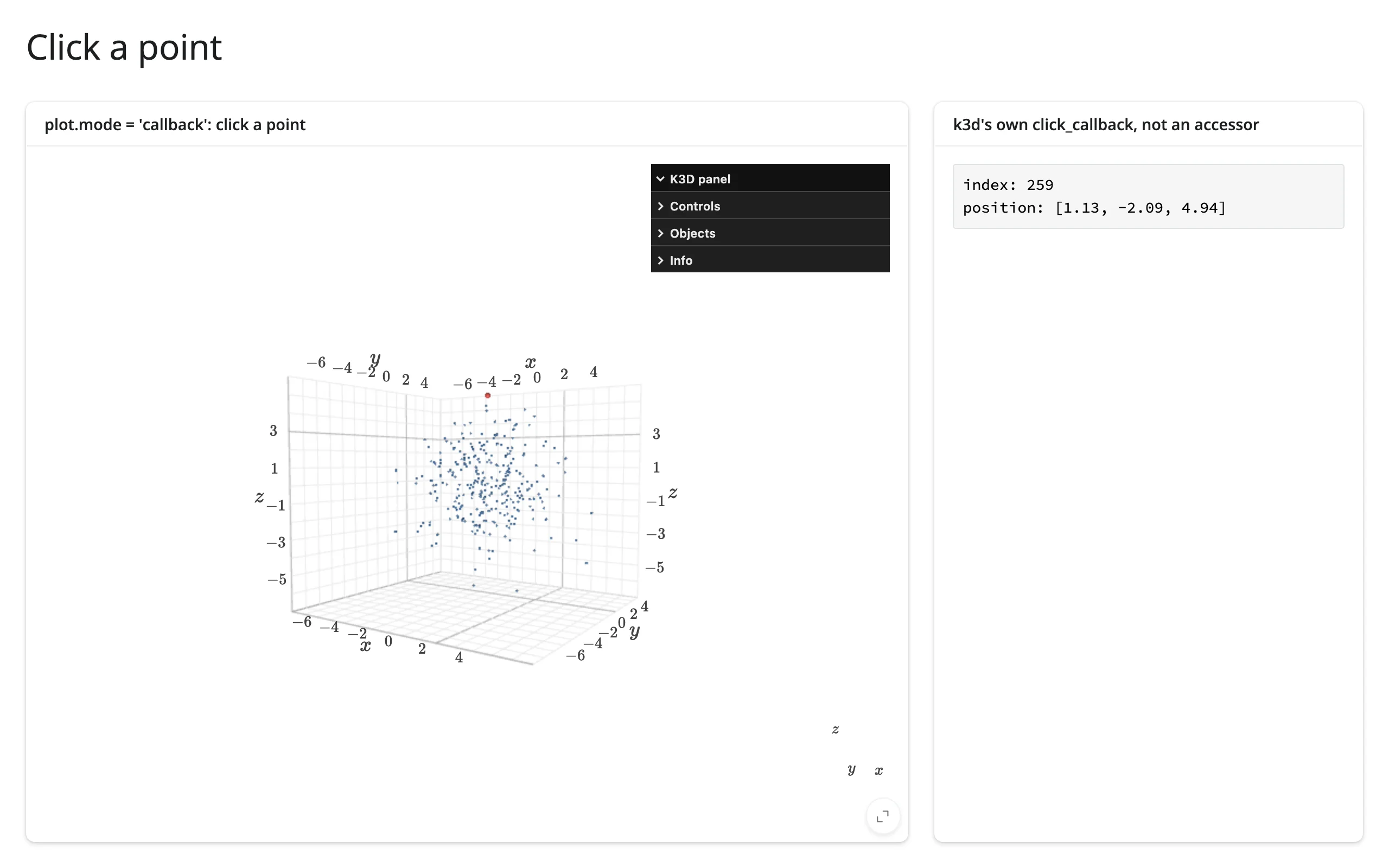
click_callback receives a dict: points give you index/position/distance/K3DIdentifier; surface/mesh give you position/normal/face_index/face/uv instead (no index – see the terrain showcase below for reading a surface pick). hover_callback has the same payload shape and fires continuously while the cursor moves, without a click. Picking needs a solid pixel: a click on a fully drawn shader="3d" ball lands reliably; a shader="flat"/"dot" sprite’s antialiased edge can miss (use bigger points, or "3d", for click targets).

Beyond picking, a few traits are worth reading with plot.read("trait") directly rather than an accessor – it’s the same widget camera() reads from, just by name, with no post-processing:

• time – during start_auto_play(), plot.read("time") updates continuously (K3D ticks it at plot.fps, default 25/s). See Rate limiting below for taming that.
• screenshot – call plot.widget.fetch_screenshot(), then plot.read("screenshot") returns a base64 PNG once the browser responds (verified: ~400KB for a simple scene, 2x screenshot_scale by default). There’s no accessor for this because it’s one-shot, not a stream.
• Menu-panel edits – toggling gridVisible/cameraAutoFit/etc. in K3D’s own on-canvas panel syncs back: plot.read("grid_visible") changes when a user toggles it there (verified on current main).

Rate limiting

camera() has no default rate policy – K3D already throttles camera updates to roughly once per 200ms upstream, so there is nothing useful left for rate_policy/rate_delay to add to it. They matter for a plain .read("trait") on a fast-changing trait instead, like time during autoplay:

examples/10_rate_limiting.py70 lines

# camera() has no default rate policy (k3d already throttles camera updates to
# ~200ms upstream), so `rate_policy`/`rate_delay` have nothing to add there.
# They do matter for a plain .read() on a fast-changing trait, like "time"
# during autoplay (k3d ticks it at its own `fps`, default 25/s).
from __future__ import annotations

import k3d
import numpy as np
from shiny import reactive
from shiny.express import input, render, ui
from shinywidgets import render_k3d


def make_scene() -> k3d.Plot:
    rng = np.random.default_rng(0)
    xyz = (rng.normal(size=(200, 3))).astype(np.float32)
    plot = k3d.plot(grid_visible=False, menu_visibility=False)
    plot += k3d.points(xyz, point_size=0.15, color=0x4C78A8)
    return plot


ui.page_opts(title="plot.read('time') during autoplay: live vs. throttled", fillable=True)
ui.input_action_button("play", "Play both")
live_n = reactive.value(0)
throttled_n = reactive.value(0)

with ui.layout_columns():
    with ui.card():
        "Default: every tick"

        @render_k3d
        def live():
            return make_scene()

        @reactive.effect
        @reactive.event(input.play)
        def _play_live():
            live.widget.start_auto_play()

        @reactive.effect
        def _count_live():
            live.read("time")
            with reactive.isolate():
                live_n.set(live_n() + 1)

        @render.text
        def n_live():
            return f"read() fired {live_n()} times"

    with ui.card():
        "rate_delay=0.5: throttled to 2/s"

        @render_k3d(rate_policy="throttle", rate_delay=0.5)
        def throttled():
            return make_scene()

        @reactive.effect
        @reactive.event(input.play)
        def _play_throttled():
            throttled.widget.start_auto_play()

        @reactive.effect
        def _count_throttled():
            throttled.read("time")
            with reactive.isolate():
                throttled_n.set(throttled_n() + 1)

        @render.text
        def n_throttled():
            return f"read() fired {throttled_n()} times"

The same 5 seconds of autoplay fires .read("time") about 200 times unthrottled vs. 11 times with rate_delay=0.5 (re-measured on current main; the exact counts vary run to run with system load, but the ~18x gap between unthrottled and throttled is the point):

rate limiting comparison

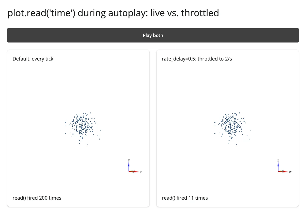
rate_policy/rate_delay on @render_k3d apply to every .read()/reactive_read() call on that widget (not just one trait), since they’re keyed by the widget instance, not the trait name – keep a fast-changing trait like time on its own widget if you need other traits read at full speed from the same scene.

Updating the widget from Python

Re-rendering rebuilds the scene from scratch: the camera resets to its auto-fit default (or whatever you set in the render function), and every object is recreated. Prefer it when the shape of the scene genuinely changes (a different object count or type).

For everything else – resizing points, recoloring, moving things – read inputs under reactive.isolate() in the render function and mutate .widget.objects[i].<trait> from a @reactive.effect. This preserves the camera and never re-sends K3D’s JS bundle:

examples/11_update_in_place.py27 lines

from __future__ import annotations

import k3d
import numpy as np
from shiny import reactive
from shiny.express import input, ui
from shinywidgets import render_k3d

rng = np.random.default_rng(0)
xyz = (rng.normal(size=(20_000, 3))).astype(np.float32)

ui.page_opts(title="Resize points without rebuilding the scene", fillable=True)
ui.input_slider("point_size", "Point size", min=0.02, max=0.3, value=0.08)


@render_k3d
def scene():
    # The render function never reads point_size, so this never re-runs:
    # orbit/zoom survive every slider move.
    plot = k3d.plot()
    plot += k3d.points(xyz, point_size=0.08, color=0x4C78A8, shader="3d")
    return plot


@reactive.effect
def _resize():
    scene.widget.objects[0].point_size = input.point_size()

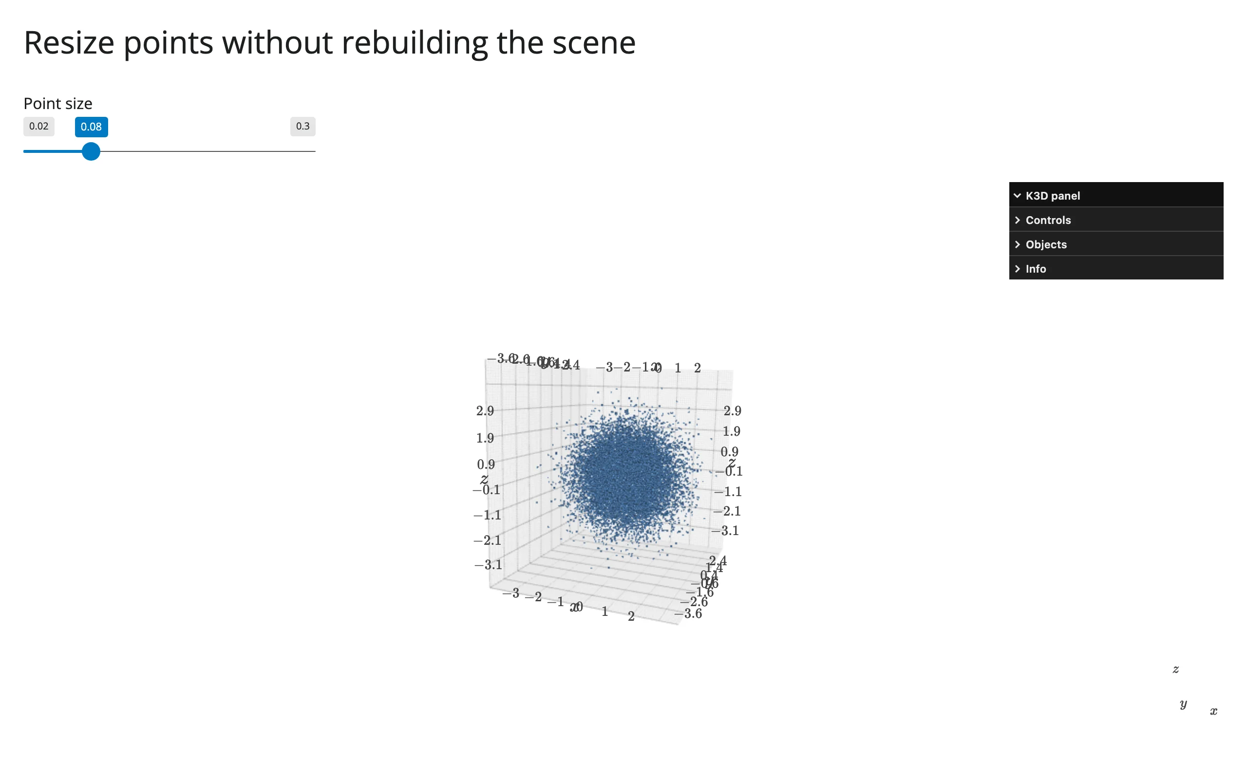
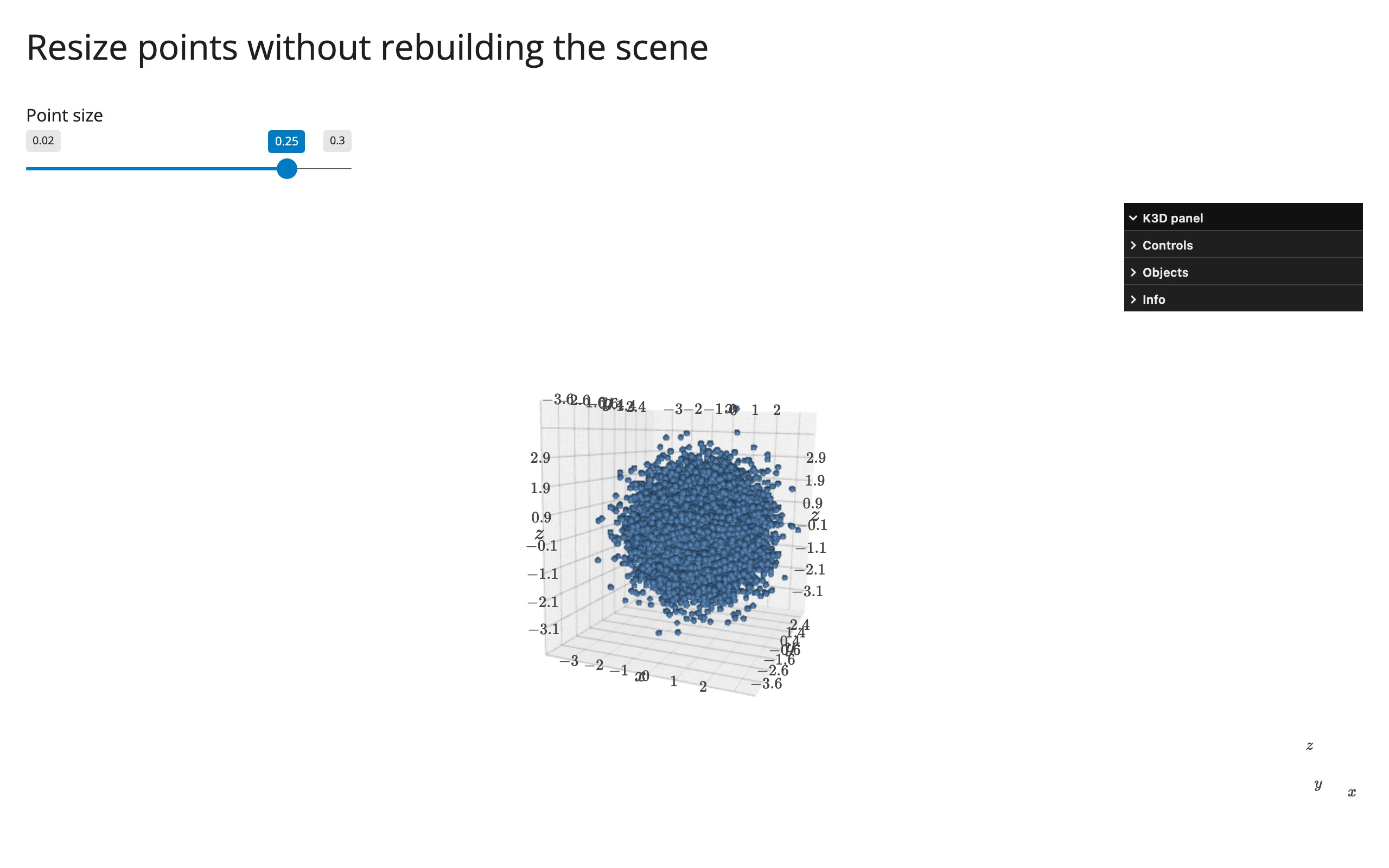
Orbited, then the slider moved from 0.08 to 0.25 – the camera is untouched:

The camera is itself just a trait, so the same pattern flies the view to a new target without resetting anything else – set plot.widget.camera = [eye_xyz, target_xyz, up_xyz] (9 floats) from an effect:

examples/12_fly_to.py52 lines

# Needs scikit-learn for the iris dataset:
#   uv run --with scikit-learn shiny run docs/widget-guides/k3d/examples/12_fly_to.py
from __future__ import annotations

import k3d
import numpy as np
from shiny import reactive
from shiny.express import input, ui
from sklearn.datasets import load_iris
from shinywidgets import render_k3d

iris = load_iris(as_frame=True).frame
xyz = iris[["sepal length (cm)", "sepal width (cm)", "petal length (cm)"]].to_numpy(np.float32)
species_color = np.choose(iris["target"].to_numpy(), [0xE41A1C, 0x377EB8, 0x4DAF4A]).astype(np.uint32)
species_names = ["setosa", "versicolor", "virginica"]
centroids = {name: xyz[iris["target"] == i].mean(axis=0) for i, name in enumerate(species_names)}
HOME = [10, -6, 6, 5.8, 3.0, 3.8, 0, 0, 1]

ui.page_opts(title="Fly to a species", fillable=True)
with ui.layout_columns():
    ui.input_action_button("home", "Home")
    for name in species_names:
        ui.input_action_button(name, name.title())


with ui.card(full_screen=True):

    @render_k3d
    def scene():
        plot = k3d.plot(camera_auto_fit=False)
        plot.camera = HOME
        plot += k3d.points(xyz, colors=species_color, point_size=0.15, shader="3d")
        return plot


@reactive.effect
@reactive.event(input.home)
def _fly_home():
    scene.widget.camera = HOME


def make_fly_to(name: str):
    @reactive.effect
    @reactive.event(getattr(input, name))
    def _fly():
        cx, cy, cz = (float(v) for v in centroids[name])
        scene.widget.camera = [cx + 2, cy - 2, cz + 2, cx, cy, cz, 0, 0, 1]

    return _fly


_fly_effects = [make_fly_to(name) for name in species_names]

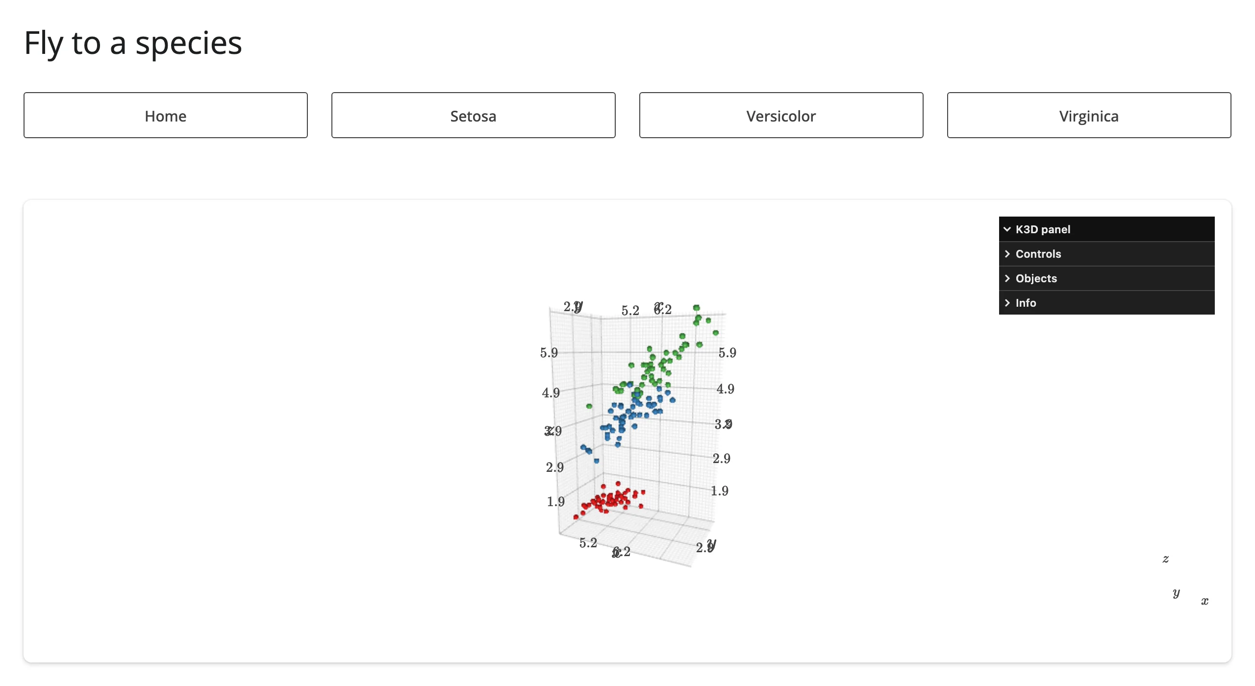
Home, then “Setosa” pressed – the camera flies to that cluster’s centroid (an instant cut here; see Gotchas for smooth easing):

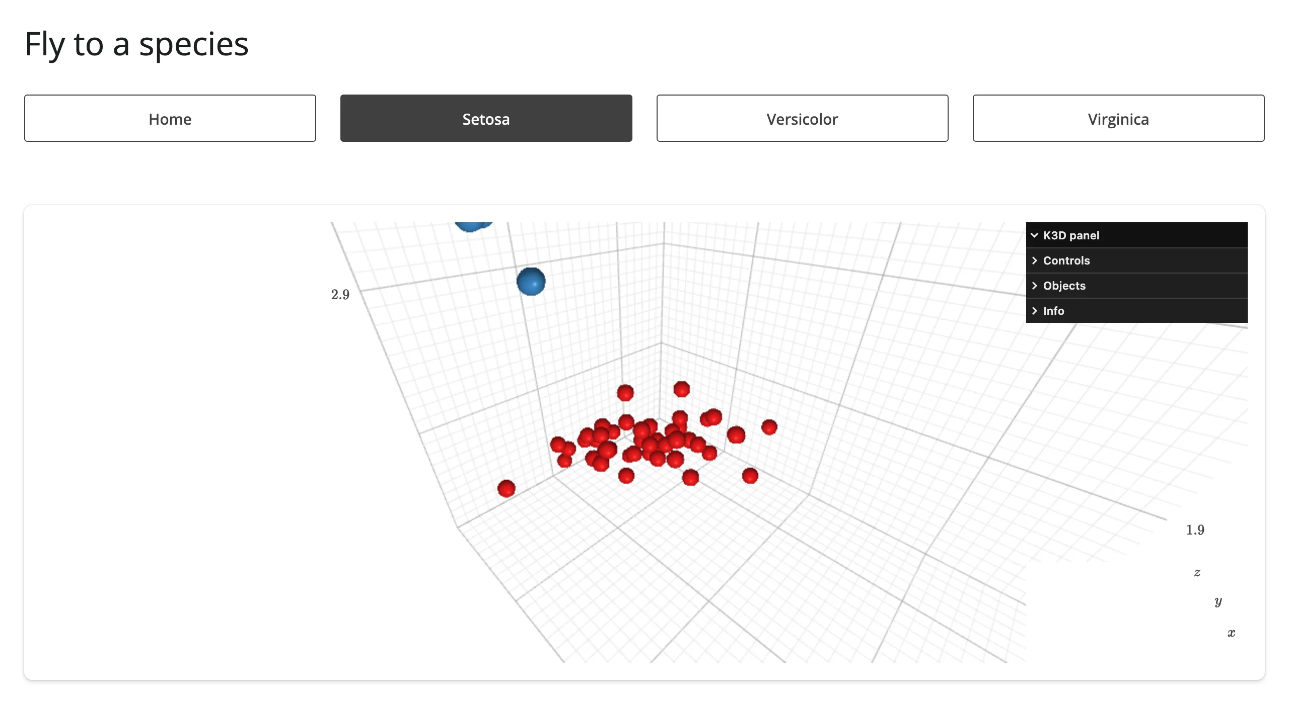
Coordinating multiple views

camera() drives a second view’s camera

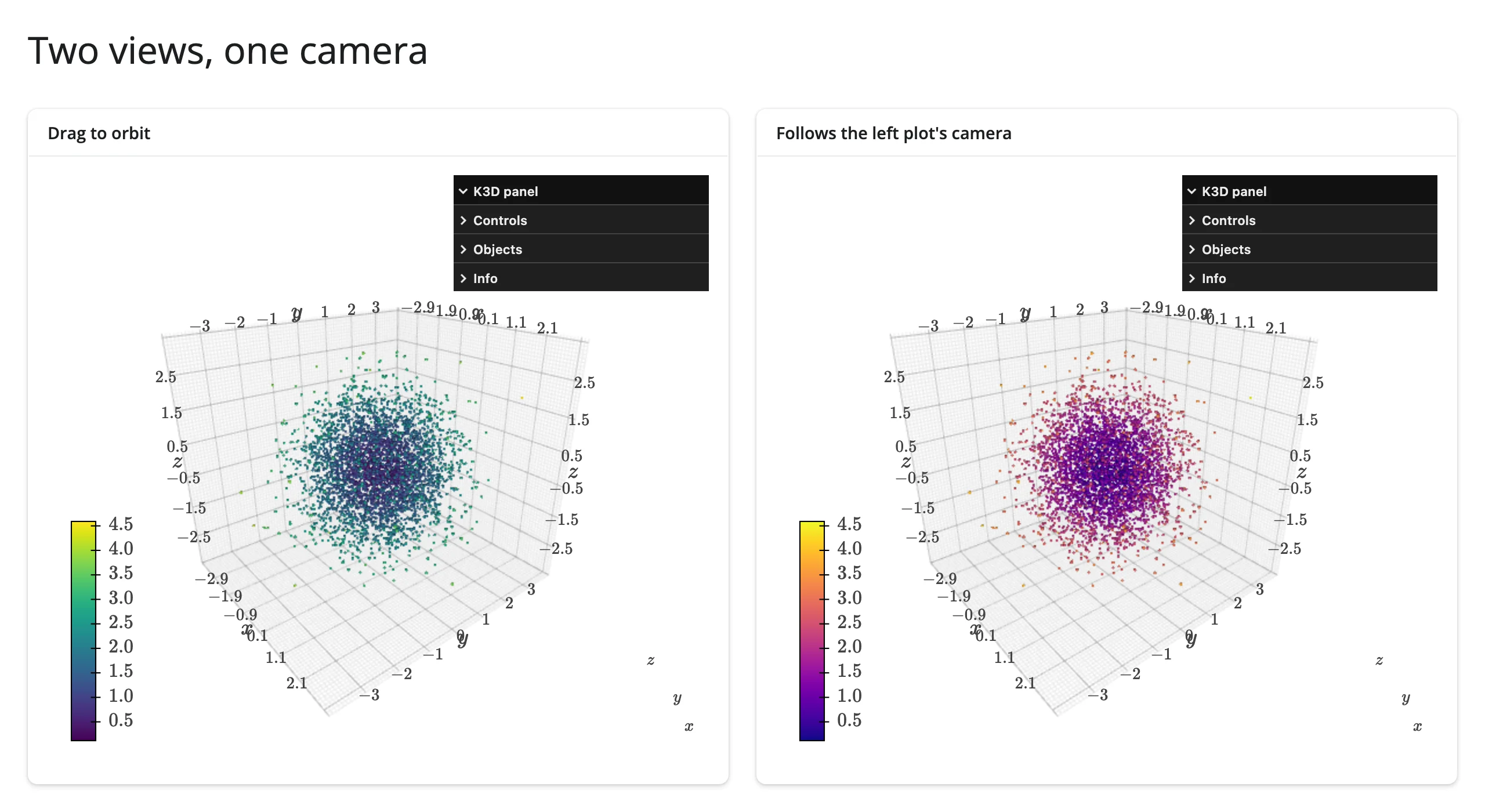
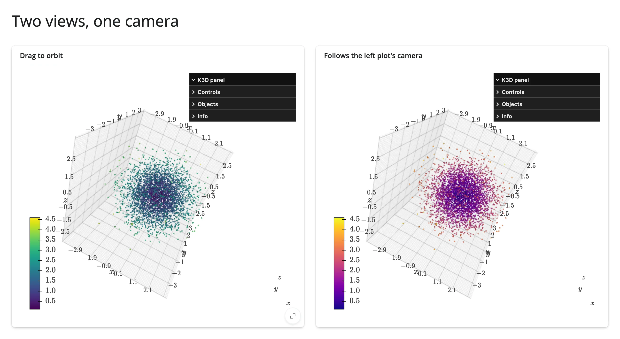
Two plots, one viewpoint: orbiting either side moves both, because the left plot’s camera() is copied straight into the right plot’s camera trait.

examples/13_sync_cameras.py50 lines

# camera() isn't just for display -- it can drive a second view directly, so
# two k3d plots stay in lockstep as you orbit either one. Try panning the
# left plot and watch the right one (lit from the opposite side) follow.
from __future__ import annotations

import k3d
import numpy as np
from shiny import reactive
from shiny.express import ui
from shinywidgets import render_k3d

rng = np.random.default_rng(0)
xyz = (rng.normal(size=(4000, 3))).astype(np.float32)
dist = np.linalg.norm(xyz, axis=1)
# Give both plots the same starting camera explicitly, rather than relying on
# auto-fit: camera() seeds its first value very early (before either plot's
# comm has opened), so the very first copy from left to right can be dropped
# (see Gotchas). Starting both plots alike means that dropped first copy is
# never visible -- every copy after a real orbit lands normally.
START = [10, -8, 6, 0, 0, 0, 0, 0, 1]

ui.page_opts(title="Two views, one camera", fillable=True)

with ui.layout_columns():
    with ui.card(full_screen=True):
        ui.card_header("Drag to orbit")

        @render_k3d
        def left():
            plot = k3d.plot(camera_auto_fit=False)
            plot.camera = START
            plot += k3d.points(xyz, point_size=0.08, attribute=dist, color_map=k3d.matplotlib_color_maps.Viridis)
            return plot

    with ui.card(full_screen=True):
        ui.card_header("Follows the left plot's camera")

        @render_k3d
        def right():
            plot = k3d.plot(camera_auto_fit=False)
            plot.camera = START
            plot += k3d.points(xyz, point_size=0.08, attribute=dist, color_map=k3d.matplotlib_color_maps.Plasma)
            return plot


@reactive.effect
def _sync():
    camera = left.camera()
    with reactive.isolate():
        right.widget.camera = camera

Before and after orbiting the left plot:

Click a point, select its row in a table

Pairs with: itables, reactable (either renders the same pd.DataFrame directly). Picking a point calls K3D’s own click_callback, which sets the row selection on a core Shiny render.data_frame:

examples/14_click_to_table.py48 lines

# Pairs with: itables, reactable (swap render.data_frame for either).
from __future__ import annotations

import k3d
import numpy as np
import pandas as pd
from shiny import reactive
from shiny.express import render, ui
from shinywidgets import render_k3d

rng = np.random.default_rng(1)
xyz = (rng.normal(size=(20, 3))).astype(np.float32)
df = pd.DataFrame(xyz.astype(np.float64), columns=["x", "y", "z"]).round(2)

clicked_index = reactive.value(None)

ui.page_opts(title="Click a point, select its row", fillable=True)

with ui.layout_columns(col_widths=[7, 5]):
    with ui.card(full_screen=True):
        ui.card_header("plot.mode = 'callback'")

        @render_k3d
        def scene():
            plot = k3d.plot(mode="callback")
            plot += k3d.points(
                xyz,
                point_size=0.12,
                color=0x4C78A8,
                click_callback=lambda info: clicked_index.set(info["index"]),
            )
            return plot

    with ui.card(full_screen=True):
        ui.card_header("Matching row, selected")

        @render.data_frame
        def table():
            return render.DataGrid(df, selection_mode="row")


# A DataGrid's row selection is driven from the server with
# update_cell_selection() (async, so this effect must be too).
@reactive.effect
async def _select():
    idx = clicked_index()
    if idx is not None:
        await table.update_cell_selection({"type": "row", "rows": (idx,)})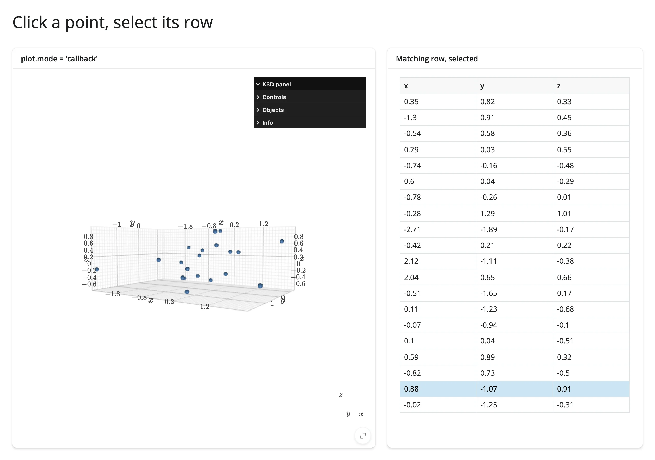

click to table

A table drives the camera

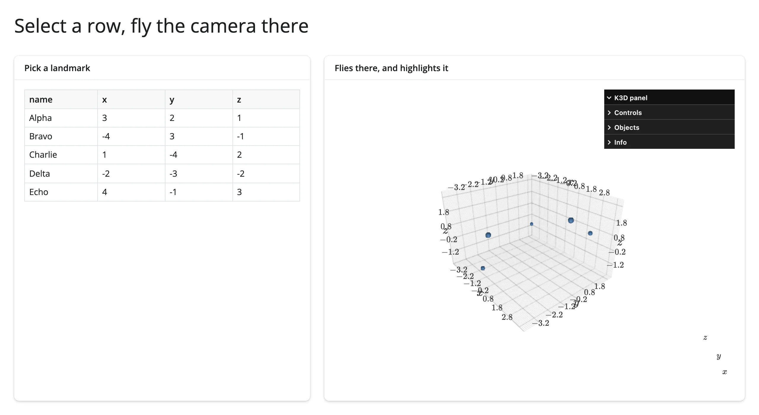
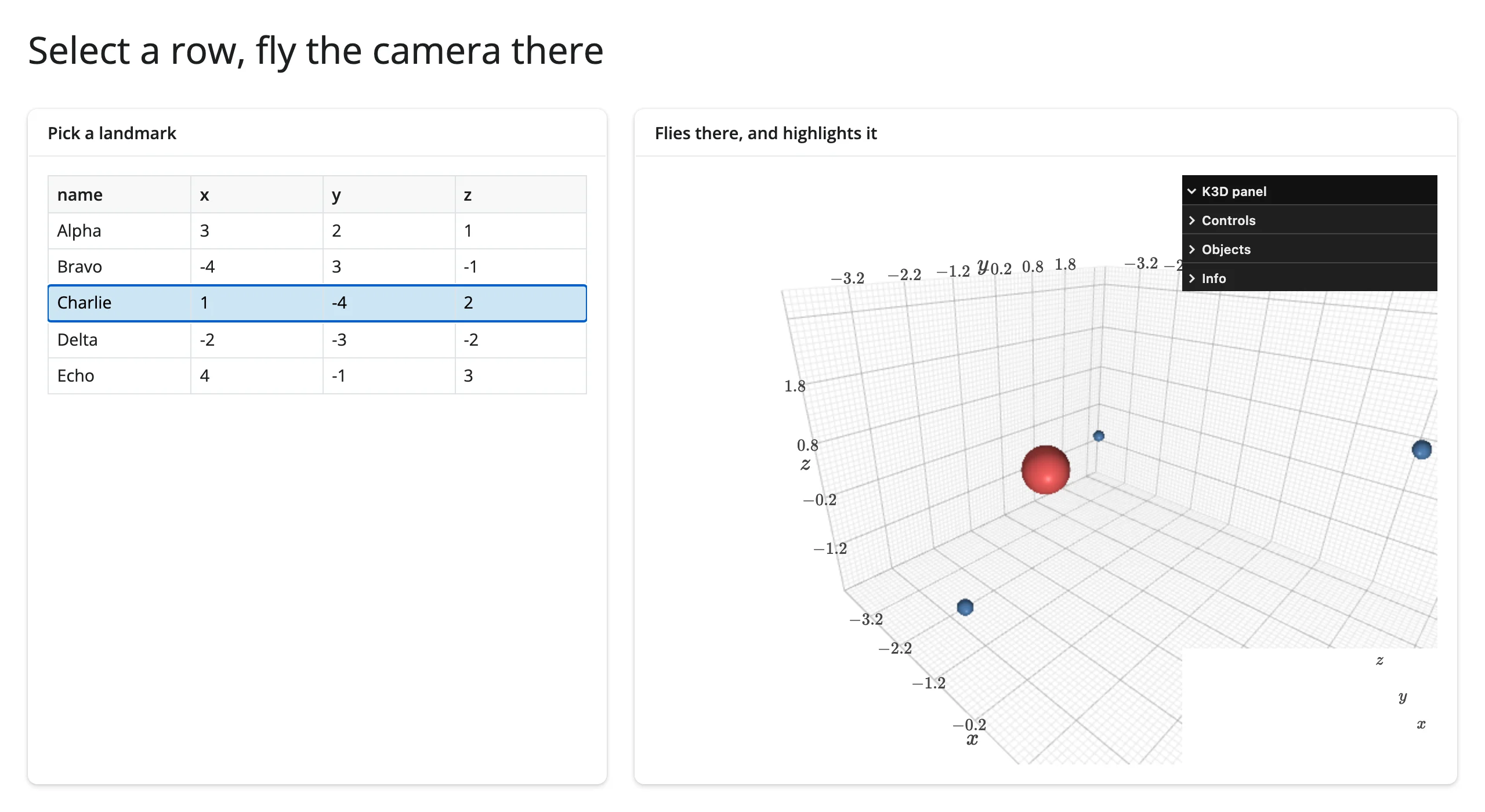
The reverse pairing: selecting a row in a plain render.DataGrid flies the camera to that landmark and highlights it – this direction needs no workaround, because the browser’s own row-click is what starts the reactive flow (the effect below runs no differently than any other input-driven effect in this guide).

examples/15_table_to_fly_to.py54 lines

# Pairs with: itables, reactable (swap render.data_frame for either).
from __future__ import annotations

import k3d
import numpy as np
import pandas as pd
from shiny import reactive
from shiny.express import render, ui
from shinywidgets import render_k3d

landmarks = pd.DataFrame(
    {
        "name": ["Alpha", "Bravo", "Charlie", "Delta", "Echo"],
        "x": [3.0, -4.0, 1.0, -2.0, 4.0],
        "y": [2.0, 3.0, -4.0, -3.0, -1.0],
        "z": [1.0, -1.0, 2.0, -2.0, 3.0],
    }
)
xyz = landmarks[["x", "y", "z"]].to_numpy(np.float32)
HOME = [12, -10, 8, 0, 0, 0, 0, 0, 1]

ui.page_opts(title="Select a row, fly the camera there", fillable=True)

with ui.layout_columns(col_widths=[5, 7]):
    with ui.card():
        ui.card_header("Pick a landmark")

        @render.data_frame
        def table():
            return render.DataGrid(landmarks, selection_mode="row")

    with ui.card(full_screen=True):
        ui.card_header("Flies there, and highlights it")

        @render_k3d
        def scene():
            plot = k3d.plot(camera_auto_fit=False)
            plot.camera = HOME
            plot += k3d.points(xyz, point_size=0.3, color=0x4C78A8, shader="3d")
            plot += k3d.points(xyz[:1], point_size=0.45, color=0xE45756, visible=False)
            return plot


@reactive.effect
def _fly_to_selection():
    sel = table.cell_selection()["rows"]
    if not sel:
        return
    idx = sel[0]
    x, y, z = (float(v) for v in xyz[idx])
    scene.widget.camera = [x + 3, y - 3, z + 2, x, y, z, 0, 0, 1]
    highlight = scene.widget.objects[1]
    highlight.positions = xyz[idx : idx + 1]
    highlight.visible = True

“Charlie” selected – the camera flew to it and the point lit up red:

Large data

K3D draws with the GPU (WebGL via three.js), so it’s the “draw it with the GPU in the browser” entry in Large data & performance’s three approaches. shader="flat" billboard sprites (see examples/02_point_cloud_scale.py in “What you can build” above) are the fast path at scale: a million points stayed orbitable at interactive frame rates, verified on current main even under SwiftShader software rendering with no real GPU. K3D doesn’t decimate, chunk, or level-of-detail a cloud for you past that – for tens of millions of points you’d thin the data in Python before handing it to k3d.points().

Layout and sizing

A plot fills its output by default. k3d.plot(height=N) (any N other than K3D’s own default of 512) opts out of filling and renders at that fixed pixel height instead; so does an ipywidgets.Layout(height="...") assigned to plot.layout – both are honored without clipping or overflow (verified on current main; this was previously broken – see Gotchas for what changed).

examples/16_layout_sizing.py43 lines

from __future__ import annotations

import k3d
import numpy as np
from ipywidgets import Layout
from shiny.express import ui
from shinywidgets import render_k3d

rng = np.random.default_rng(0)
xyz = (rng.random((200, 3), dtype=np.float32))


def make_plot(**kwargs) -> k3d.Plot:
    plot = k3d.plot(**kwargs)
    plot += k3d.points(xyz, point_size=0.05, color=0x4C78A8)
    return plot


ui.page_opts(title="Sizing", fillable=True)

with ui.layout_columns():
    with ui.card(full_screen=True):
        "Fills its card (no explicit height) -- try full_screen"

        @render_k3d
        def fills():
            return make_plot()

    with ui.card():
        "Fixed height via k3d.plot(height=250)"

        @render_k3d
        def fixed_height():
            return make_plot(height=250)

    with ui.card():
        "Fixed height via ipywidgets Layout(height='250px')"

        @render_k3d
        def layout_height():
            plot = make_plot()
            plot.layout = Layout(height="250px")
            return plot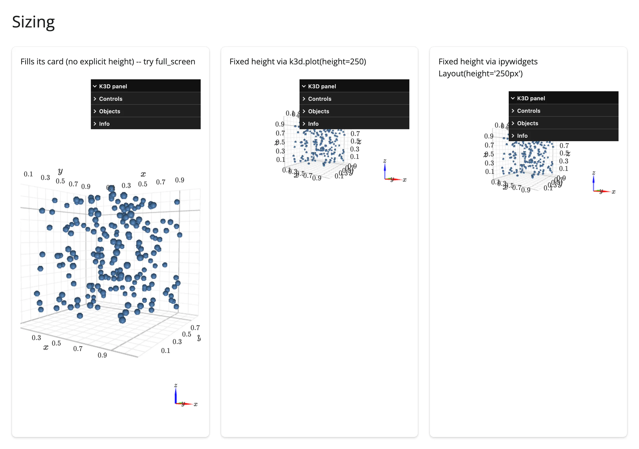

layout and sizing

Measured: the fill card’s canvas tracks its card exactly; both fixed-height variants render at exactly 250px, with no clipped or overflowing content either way.

Gotchas and limitations

Verified on current main (shinywidgets commit 32ca7035, k3d 3.2.0, shiny 1.9.0):

• start_auto_play() called before the k3d view connects is dropped silently. A .send()-backed call (e.g. scene.start_auto_play()) made inside the render function is now delivered to the browser instead of being dropped by shinywidgets – confirmed with a websocket capture. But k3d’s own JS registers its custom-message handler per view, at view-connect time, so a message that arrives earlier (the render function, or a bare startup effect on a slow page) is lost for good: playback never starts, with no error anywhere. Once the view is connected, server-initiated calls work with no user gesture needed (verified: an effect delayed ~5 s via reactive.invalidate_later() starts playback). Even so, wire start_auto_play()/stop_auto_play() to buttons, as examples/07_animation.py does – a click always lands after the view is up, however slow the page.
• k3d.text’s default LaTeX rendering drops spaces. k3d.text("Highest point (1068 m)") renders as “Highestpoint(1068m)” – text is KaTeX by default, which strips plain spaces. Pass is_html=True (as the terrain example does) or escape spaces as \.
• There is no clicked() accessor, by design. Picking requires plot.mode = "callback", a visible change to the plot’s interaction mode, which this design’s accessor model won’t make silently. See “Beyond the accessors.”
• marching_cubes ignores your field’s coordinate range. The isosurface always comes out in a unit cube centered on the origin, regardless of the linspace range used to build the field – rescale with spacings_x/_y/_z or a model_matrix if you need it in your own coordinate system.
• fetch_screenshot() 404s on KaTeX font files. The screenshot path re-requests relative fonts/KaTeX_*.woff/.ttf URLs that resolve against the Shiny app’s origin instead of k3d’s bundled fonts. Live rendering is unaffected (the fonts are already loaded as inline data URLs); this only shows up as harmless 404s in the browser console during a screenshot capture. Upstream k3d behavior, not a shinywidgets bug.
• camera_auto_fit’s margin is generous. The default camera frames data with real whitespace around it (camera_reset()’s default factor=1.5); for a tighter, more deliberate composition (e.g. a hero screenshot or gallery app), set camera_auto_fit=False and an explicit plot.camera instead of relying on auto-fit.
• Camera moves set this way are instant cuts, not smooth flights. plot.widget.camera = [...] jumps directly to the new view. K3D has no built-in camera tween; if you want eased motion, interpolate the 9 numbers yourself across a few reactive.invalidate_later() ticks, or accept the cut (it still reads clearly as “flying to X” in context, per the fly-to example above).

What we deliberately didn’t chase further: the old report’s re-render comm/model leak (finding 3.1, k3d’s Plot.close() not calling super().close()) is fixed on current main with a shim (close_comm_on_close() in _shinywidgets.py) – confirmed by reading the code, not independently re-measured with the old report’s exact 8-re-render repro. The old report’s Layout(height=) clipping claim (finding 3.2) is also fixed, and is re-verified here (see Layout and sizing above, examples/16_layout_sizing.py).

Gallery candidates

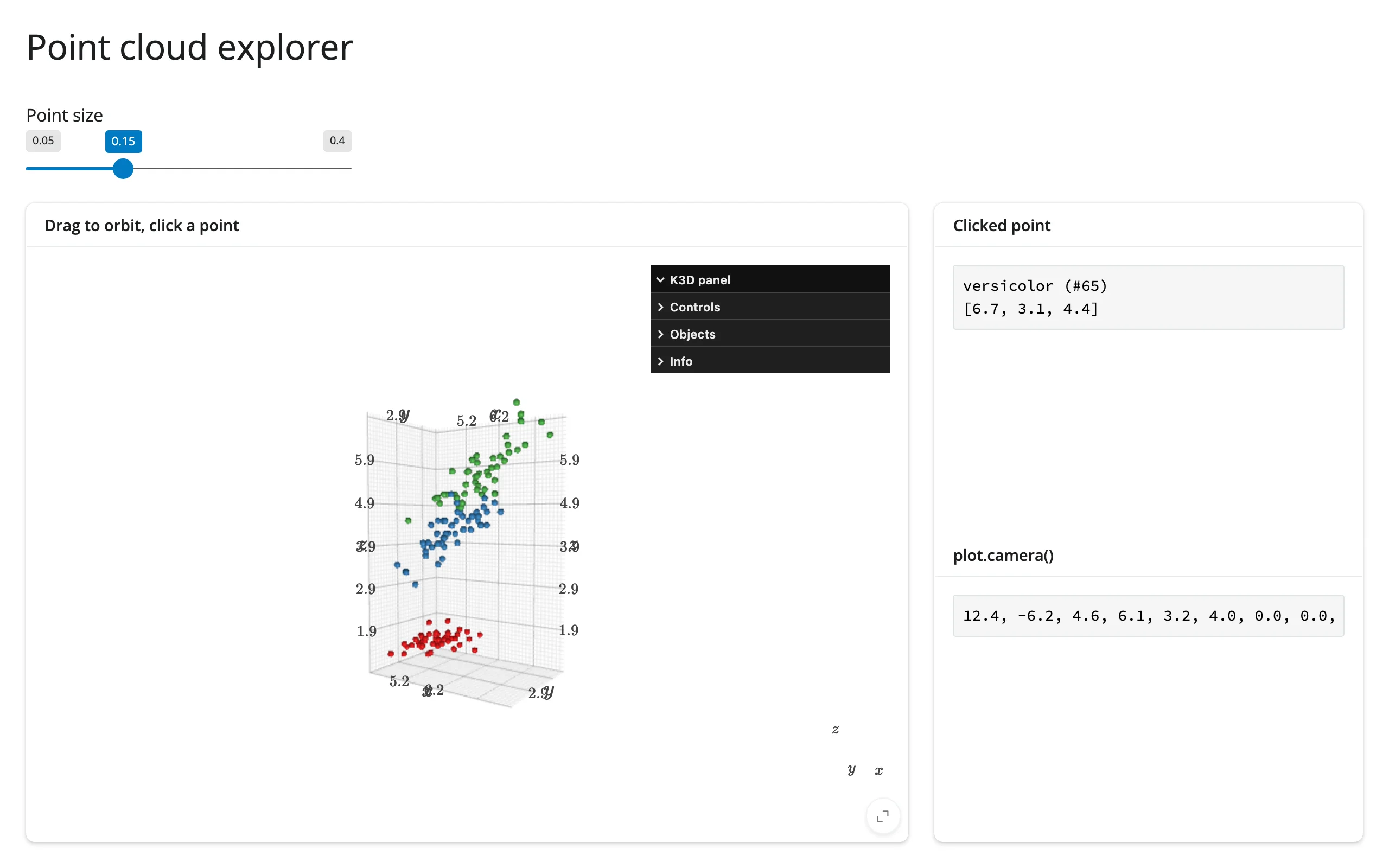
template_point_cloud_explorer.py

A small, adaptable starting point (bucket: template): orbit, resize points live, click a point for details, and read the camera – swap in your own (n, 3) array and labels. Uses the iris dataset in 3D, colored by species.

gallery template

showcase_terrain_explorer.py

A fuller demo (bucket: showcase): the same real Jacksboro Fault DEM from above, now with plot.mode = "callback" picking (click anywhere to read elevation in meters, resolved from the nearest grid cell via the surface pick’s position), “fly to highest/lowest point” buttons, a live camera readout, and a wireframe toggle that restyles the surface in place.

Learn more

• K3D Jupyter documentation and its example gallery (Jupyter notebooks; the API is identical in Shiny)
• K3D factory function reference (k3d.points, k3d.surface, k3d.volume, k3d.marching_cubes, k3d.vectors, k3d.text, and more)
• Related guides in this roster: plotly (scatter_3d, lighter-weight 3D), pythreejs (lower-level three.js scene graph), lonboard and niivue (domain-specific 3D: geospatial, medical imaging), itables / reactable (used above for the linked table patterns)